Overview
Most chapters of this Cookbook leverage a 12-hour subset of ERA5 data, using two NetCDF data files that have been embedded in the Cookbook source repository. The purpose of this notebook is to demonstrate how to reproduce and extend a feature tracking result by streaming data from a cloud-based ERA5 data store.
We will be streaming some cloud-formatted ERA5 data from the NCAR’s Geoscience Data Exchange. We will access the data via the Open Science Data Federation (OSDF) following guidance from the OSDF Cookbook Hampapura et al., 2025.
Our prepackaged example data
We have 12 hours of hourly sea level pressure data extracted from ERA5
import xarray as xrds = xr.open_dataset("data/SLP_ex.nc")
da = ds["SLP"]
daA reference plot
Just plot the first time step
ref_time = da.time[0]da.sel(time=ref_time).plot()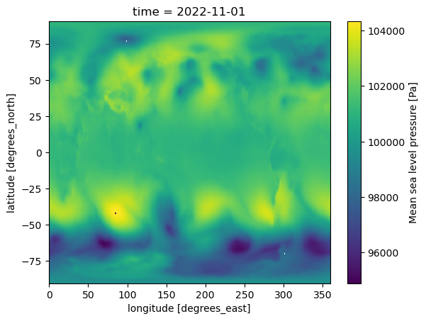
Streaming ERA5 from NSF NCAR GDEX via OSDF
To access the streaming version of the data, we are following the chapter Using PelicanFS via FSSpec to Access Data on the OSDF from the OSDF Cookbook Hampapura et al., 2025.
This method of streaming the data over OSDF relies on a tool called PelicanFS that provides a layer of robustness for network issues. Note that pelicanfs must be install in the Python environment in order for the code below to work.
path = 'osdf:///ncar/gdex/d633000/e5.oper.an.sfc.zarr/e5.oper.an.sfc.msl.zarr'
msl = xr.open_dataset(path, engine='zarr')
mslmsl.MSL.sel(time=da.time)Recreate the reference figure
msl.MSL.sel(time=ref_time).plot()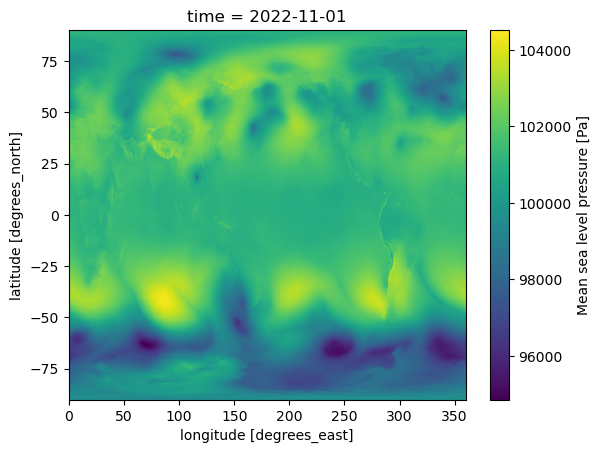
Extend a feature tracking workflow in time with streamed data
Here I’m copying code from the SLP scikit notebook but pulling the data from GDEX and extending the time range
import numpy as np
import xarray as xr
import matplotlib.pyplot as plt
from matplotlib.animation import FuncAnimation
from IPython.display import HTML
from skimage.measure import label, regionprops
import matplotlib.colors as mcolors
from matplotlib.cm import ScalarMappable
import cartopy.crs as ccrs
This just pulls in a 48-hour slice of data, including the 12 hours from our example dataset.
da = msl.MSL.sel(time=slice('2022-11-01','2022-11-02'))
daEverything that follows is taken straight from the other notebook
threshold = 100000
min_area = 20
min_overlap = 0.2


# ---- get lat/lon coords ----
# assumes dims like (time, lat, lon)
lat = da[da.dims[1]].values
lon = da[da.dims[2]].values

# if lat/lon are 1D, make 2D grids for contourf/contour
lon2d, lat2d = np.meshgrid(lon, lat)

def detect_features(field, threshold=100000, min_area=20):
    mask = field <= threshold
    labels = label(mask, connectivity=2)

    for lab in np.unique(labels)[1:]:
        if np.sum(labels == lab) < min_area:
            labels[labels == lab] = 0

    labels = label(labels > 0, connectivity=2)
    return labels

# ---- precompute tracked features ----
tracked = []
prev = {}
next_track_id = 1

for t in range(da.sizes["time"]):
    field = da.isel(time=t).values
    labels = detect_features(field, threshold=threshold, min_area=min_area)

    current = {}
    frame_info = []

    for r in regionprops(labels):
        mask = labels == r.label

        best_id = None
        best_overlap = 0.0

        for track_id, old_mask in prev.items():
            overlap = np.logical_and(mask, old_mask).sum() / mask.sum()
            if overlap > best_overlap:
                best_overlap = overlap
                best_id = track_id

        if best_overlap < min_overlap:
            best_id = next_track_id
            next_track_id += 1

        current[best_id] = mask
        frame_info.append({
            "track_id": best_id,
            "centroid_rc": r.centroid,   # row, col
            "mask": mask
        })

    tracked.append(frame_info)
    prev = current


def update(t):
    ax.clear()

    field = da.isel(time=t).values

    # SLP as colored contour lines, not filled
    cs = ax.contour(
        lon2d, lat2d, field,
        levels=levels,
        cmap="turbo",          # or "rainbow", "viridis", "plasma"
        linewidths=0.9,
        transform=ccrs.PlateCarree()
    )

    # tracked feature outlines + labels
    for feat in tracked[t]:
        mask = feat["mask"]

        ax.contour(
            lon2d, lat2d, mask.astype(int),
            levels=[0.5],
            colors="black",
            linewidths=1.6,
            transform=ccrs.PlateCarree()
        )

        y, x = feat["centroid_rc"]
        iy = int(round(y))
        ix = int(round(x))

        ax.plot(
            lon[ix], lat[iy],
            "ko", ms=3,
            transform=ccrs.PlateCarree()
        )

        ax.text(
            lon[ix], lat[iy],
            str(feat["track_id"]),
            fontsize=8,
            color="black",
            ha="left",
            va="bottom",
            transform=ccrs.PlateCarree(),
            bbox=dict(facecolor="white", edgecolor="none", alpha=0.7, pad=1)
        )

    # continents/coastlines: faint, not black
    ax.coastlines(color="0.55", linewidth=0.6)

    # faint gridlines
    gl = ax.gridlines(
        draw_labels=True,
        linewidth=0.4,
        color="0.5",
        alpha=0.25,
        linestyle="--"
    )
    gl.top_labels = False
    gl.right_labels = False

    ax.set_title(f"Scikit tracked SLP features | time index = {t}")
# ---- color scale fixed across all frames ----
vmin = float(da.min())
vmax = float(da.max())
levels = np.linspace(vmin, vmax, 16)
norm = mcolors.Normalize(vmin=vmin, vmax=vmax)
cmap = "turbo"


# ---- animate ----
fig, ax = plt.subplots(figsize=(8, 4), subplot_kw={"projection": ccrs.PlateCarree()})

sm = ScalarMappable(norm=norm, cmap=cmap)
sm.set_array([])
cbar = fig.colorbar(sm, ax=ax, pad=0.02)
cbar.set_label("SLP")


anim = FuncAnimation(
    fig,
    update,
    frames=da.sizes["time"],
    interval=300,
    blit=False,
)

plt.close(fig)
HTML(anim.to_jshtml())Same animation, but now over 48 hours!
- Hampapura, H. R., Hoelzemann, A., Wall, C., Panta, A., Schuster, D., Kent, J., Turetsky, E. T., Wingert Barok, A., Bockelman, B., Hiemstra, J. T., Conroy, R. P., Del Vecchio, J., Koech, K., & OSDF cookbook contributors. (2025). OSDF Cookbook. Zenodo. 10.5281/ZENODO.16802784