Clouds over SGP for April 4, 2019
Looking at LASSO data for April 4, 2019 to see meterological data and calculate cloud base and cloud top.
Imports
from datetime import datetime
import numpy as np
import xarray as xr
import fsspec
import xwrf

import matplotlib.pyplot as plt
Bring in the data
Here is the raw model output from LASSO.
# Set the URL and path for the cloud
URL = 'https://js2.jetstream-cloud.org:8001/'
path = f'pythia/lasso-sgp'

# Configure the s3-like storage endpoint on jetstream
fs = fsspec.filesystem("s3", anon=True, client_kwargs=dict(endpoint_url=URL))

# Set the analysis date and simulation number
case_date = datetime(2019, 4, 4)
sim_id = 7

# Read the wrfstat files
wrfstat_pattern = f's3://{path}/sim000{sim_id}/raw_model/wrfstat*'
wrfstat_files = sorted(fs.glob(wrfstat_pattern))

# Remotely read these into a list
wrfstat_file_list = [fs.open(file) for file in wrfstat_files]
wrfstat_file_list
Load into an xarray.Dataset
ds_stat = xr.open_mfdataset(wrfstat_file_list, engine='h5netcdf')

# Rename time - in this case, we are not using xwrf to clean the dataset
ds_stat["Time"] = ds_stat["XTIME"]
ds_stat
<xarray.Dataset> Size: 72GB
Dimensions:         (Time: 91, bottom_top: 226, bottom_top_stag: 227,
                     south_north: 250, west_east: 250, west_east_stag: 251,
                     south_north_stag: 251)
Coordinates:
    XTIME           (Time) datetime64[ns] 728B dask.array<chunksize=(91,), meta=np.ndarray>
  * Time            (Time) datetime64[ns] 728B 2019-04-04T12:00:00 ... 2019-0...
Dimensions without coordinates: bottom_top, bottom_top_stag, south_north,
                                west_east, west_east_stag, south_north_stag
Data variables: (12/179)
    Times           (Time) |S19 2kB dask.array<chunksize=(1,), meta=np.ndarray>
    CST_CLDLOW      (Time) float32 364B dask.array<chunksize=(91,), meta=np.ndarray>
    CST_CLDTOT      (Time) float32 364B dask.array<chunksize=(91,), meta=np.ndarray>
    CST_LWP         (Time) float32 364B dask.array<chunksize=(91,), meta=np.ndarray>
    CST_IWP         (Time) float32 364B dask.array<chunksize=(91,), meta=np.ndarray>
    CST_PRECW       (Time) float32 364B dask.array<chunksize=(91,), meta=np.ndarray>
    ...              ...
    CSV_IWC         (Time, bottom_top, south_north, west_east) float32 5GB dask.array<chunksize=(1, 226, 125, 125), meta=np.ndarray>
    CSV_CLDFRAC     (Time, bottom_top, south_north, west_east) float32 5GB dask.array<chunksize=(1, 226, 125, 125), meta=np.ndarray>
    CSS_LWP         (Time, south_north, west_east) float32 23MB dask.array<chunksize=(1, 125, 125), meta=np.ndarray>
    CSS_IWP         (Time, south_north, west_east) float32 23MB dask.array<chunksize=(1, 125, 125), meta=np.ndarray>
    CSS_CLDTOT      (Time, south_north, west_east) float32 23MB dask.array<chunksize=(1, 125, 125), meta=np.ndarray>
    CSS_CLDLOW      (Time, south_north, west_east) float32 23MB dask.array<chunksize=(1, 125, 125), meta=np.ndarray>
Attributes: (12/96)
    TITLE:                                  OUTPUT FROM WRF V3.8.1 MODEL
    START_DATE:                            2019-04-04_12:00:00
    WEST-EAST_GRID_DIMENSION:              251
    SOUTH-NORTH_GRID_DIMENSION:            251
    BOTTOM-TOP_GRID_DIMENSION:             227
    DX:                                    100.0
    ...                                    ...
    config_aerosol:                        NA
    config_forecast_time:                  15.0 h
    config_boundary_method:                Periodic
    config_microphysics:                   Thompson (mp_physics=8)
    config_nickname:                       runlas20190404v1msda2d150km
    simulation_origin_host:                cumulus-login2.ccs.ornl.gov
xarray.Dataset
- Time: 91
- bottom_top: 226
- bottom_top_stag: 227
- south_north: 250
- west_east: 250
- west_east_stag: 251
- south_north_stag: 251
- XTIME(Time)datetime64[ns]dask.array<chunksize=(91,), meta=np.ndarray>
- FieldType :
- 104
- MemoryOrder :
- 0
- description :
- minutes since 2019-04-04 12:00:00
- stagger :
Array Chunk Bytes 728 B 728 B Shape (91,) (91,) Dask graph 1 chunks in 2 graph layers Data type datetime64[ns] numpy.ndarray - Time(Time)datetime64[ns]2019-04-04T12:00:00 ... 2019-04-...
- FieldType :
- 104
- MemoryOrder :
- 0
- description :
- minutes since 2019-04-04 12:00:00
- stagger :
array(['2019-04-04T12:00:00.000000000', '2019-04-04T12:10:00.000000000',
       '2019-04-04T12:20:00.000000000', '2019-04-04T12:30:00.000000000',
       '2019-04-04T12:40:00.000000000', '2019-04-04T12:50:00.000000000',
       '2019-04-04T13:00:00.000000000', '2019-04-04T13:10:00.000000000',
       '2019-04-04T13:20:00.000000000', '2019-04-04T13:30:00.000000000',
       '2019-04-04T13:40:00.000000000', '2019-04-04T13:50:00.000000000',
       '2019-04-04T14:00:00.000000000', '2019-04-04T14:10:00.000000000',
       '2019-04-04T14:20:00.000000000', '2019-04-04T14:30:00.000000000',
       '2019-04-04T14:40:00.000000000', '2019-04-04T14:50:00.000000000',
       '2019-04-04T15:00:00.000000000', '2019-04-04T15:10:00.000000000',
       '2019-04-04T15:20:00.000000000', '2019-04-04T15:30:00.000000000',
       '2019-04-04T15:40:00.000000000', '2019-04-04T15:50:00.000000000',
       '2019-04-04T16:00:00.000000000', '2019-04-04T16:10:00.000000000',
       '2019-04-04T16:20:00.000000000', '2019-04-04T16:30:00.000000000',
       '2019-04-04T16:40:00.000000000', '2019-04-04T16:50:00.000000000',
       '2019-04-04T17:00:00.000000000', '2019-04-04T17:10:00.000000000',
       '2019-04-04T17:20:00.000000000', '2019-04-04T17:30:00.000000000',
       '2019-04-04T17:40:00.000000000', '2019-04-04T17:50:00.000000000',
       '2019-04-04T18:00:00.000000000', '2019-04-04T18:10:00.000000000',
       '2019-04-04T18:20:00.000000000', '2019-04-04T18:30:00.000000000',
       '2019-04-04T18:40:00.000000000', '2019-04-04T18:50:00.000000000',
       '2019-04-04T19:00:00.000000000', '2019-04-04T19:10:00.000000000',
       '2019-04-04T19:20:00.000000000', '2019-04-04T19:30:00.000000000',
       '2019-04-04T19:40:00.000000000', '2019-04-04T19:50:00.000000000',
       '2019-04-04T20:00:00.000000000', '2019-04-04T20:10:00.000000000',
       '2019-04-04T20:20:00.000000000', '2019-04-04T20:30:00.000000000',
       '2019-04-04T20:40:00.000000000', '2019-04-04T20:50:00.000000000',
       '2019-04-04T21:00:00.000000000', '2019-04-04T21:10:00.000000000',
       '2019-04-04T21:20:00.000000000', '2019-04-04T21:30:00.000000000',
       '2019-04-04T21:40:00.000000000', '2019-04-04T21:50:00.000000000',
       '2019-04-04T22:00:00.000000000', '2019-04-04T22:10:00.000000000',
       '2019-04-04T22:20:00.000000000', '2019-04-04T22:30:00.000000000',
       '2019-04-04T22:40:00.000000000', '2019-04-04T22:50:00.000000000',
       '2019-04-04T23:00:00.000000000', '2019-04-04T23:10:00.000000000',
       '2019-04-04T23:20:00.000000000', '2019-04-04T23:30:00.000000000',
       '2019-04-04T23:40:00.000000000', '2019-04-04T23:50:00.000000000',
       '2019-04-05T00:00:00.000000000', '2019-04-05T00:10:00.000000000',
       '2019-04-05T00:20:00.000000000', '2019-04-05T00:30:00.000000000',
       '2019-04-05T00:40:00.000000000', '2019-04-05T00:50:00.000000000',
       '2019-04-05T01:00:00.000000000', '2019-04-05T01:10:00.000000000',
       '2019-04-05T01:20:00.000000000', '2019-04-05T01:30:00.000000000',
       '2019-04-05T01:40:00.000000000', '2019-04-05T01:50:00.000000000',
       '2019-04-05T02:00:00.000000000', '2019-04-05T02:10:00.000000000',
       '2019-04-05T02:20:00.000000000', '2019-04-05T02:30:00.000000000',
       '2019-04-05T02:40:00.000000000', '2019-04-05T02:50:00.000000000',
       '2019-04-05T03:00:00.000000000'], dtype='datetime64[ns]')
- Times(Time)|S19dask.array<chunksize=(1,), meta=np.ndarray>
Array Chunk Bytes 1.69 kiB 19 B Shape (91,) (1,) Dask graph 91 chunks in 2 graph layers Data type |S19 numpy.ndarray - CST_CLDLOW(Time)float32dask.array<chunksize=(91,), meta=np.ndarray>
- FieldType :
- 104
- MemoryOrder :
- 0
- description :
- Fractional low-cloud cover (<5 km)
- units :
- (0-1)
- stagger :
Array Chunk Bytes 364 B 364 B Shape (91,) (91,) Dask graph 1 chunks in 2 graph layers Data type float32 numpy.ndarray - CST_CLDTOT(Time)float32dask.array<chunksize=(91,), meta=np.ndarray>
- FieldType :
- 104
- MemoryOrder :
- 0
- description :
- Fractional cloud cover
- units :
- (0-1)
- stagger :
Array Chunk Bytes 364 B 364 B Shape (91,) (91,) Dask graph 1 chunks in 2 graph layers Data type float32 numpy.ndarray - CST_LWP(Time)float32dask.array<chunksize=(91,), meta=np.ndarray>
- FieldType :
- 104
- MemoryOrder :
- 0
- description :
- Vertical integrated liquid water path (based on ql)
- units :
- kg/m^2
- stagger :
Array Chunk Bytes 364 B 364 B Shape (91,) (91,) Dask graph 1 chunks in 2 graph layers Data type float32 numpy.ndarray - CST_IWP(Time)float32dask.array<chunksize=(91,), meta=np.ndarray>
- FieldType :
- 104
- MemoryOrder :
- 0
- description :
- Vertical integrated ice water path (based on qf)
- units :
- kg/m^2
- stagger :
Array Chunk Bytes 364 B 364 B Shape (91,) (91,) Dask graph 1 chunks in 2 graph layers Data type float32 numpy.ndarray - CST_PRECW(Time)float32dask.array<chunksize=(91,), meta=np.ndarray>
- FieldType :
- 104
- MemoryOrder :
- 0
- description :
- Vertical integrated water vapor
- units :
- kg/m^2
- stagger :
Array Chunk Bytes 364 B 364 B Shape (91,) (91,) Dask graph 1 chunks in 2 graph layers Data type float32 numpy.ndarray - CST_TKE(Time)float32dask.array<chunksize=(91,), meta=np.ndarray>
- FieldType :
- 104
- MemoryOrder :
- 0
- description :
- Vertical integrated TKE
- units :
- kg/s^2
- stagger :
Array Chunk Bytes 364 B 364 B Shape (91,) (91,) Dask graph 1 chunks in 2 graph layers Data type float32 numpy.ndarray - CST_TSAIR(Time)float32dask.array<chunksize=(91,), meta=np.ndarray>
- FieldType :
- 104
- MemoryOrder :
- 0
- description :
- Surface air temperature
- units :
- K
- stagger :
Array Chunk Bytes 364 B 364 B Shape (91,) (91,) Dask graph 1 chunks in 2 graph layers Data type float32 numpy.ndarray - CST_PS(Time)float32dask.array<chunksize=(91,), meta=np.ndarray>
- FieldType :
- 104
- MemoryOrder :
- 0
- description :
- Surface pressure
- units :
- Pa
- stagger :
Array Chunk Bytes 364 B 364 B Shape (91,) (91,) Dask graph 1 chunks in 2 graph layers Data type float32 numpy.ndarray - CST_PRECT(Time)float32dask.array<chunksize=(91,), meta=np.ndarray>
- FieldType :
- 104
- MemoryOrder :
- 0
- description :
- Total precipitation at surface
- units :
- mm/sec
- stagger :
Array Chunk Bytes 364 B 364 B Shape (91,) (91,) Dask graph 1 chunks in 2 graph layers Data type float32 numpy.ndarray - CST_SH(Time)float32dask.array<chunksize=(91,), meta=np.ndarray>
- FieldType :
- 104
- MemoryOrder :
- 0
- description :
- Surface sensible heat flux
- units :
- W/m^2
- stagger :
Array Chunk Bytes 364 B 364 B Shape (91,) (91,) Dask graph 1 chunks in 2 graph layers Data type float32 numpy.ndarray - CST_LH(Time)float32dask.array<chunksize=(91,), meta=np.ndarray>
- FieldType :
- 104
- MemoryOrder :
- 0
- description :
- Surface latent heat flux
- units :
- W/m^2
- stagger :
Array Chunk Bytes 364 B 364 B Shape (91,) (91,) Dask graph 1 chunks in 2 graph layers Data type float32 numpy.ndarray - CST_FSNTC(Time)float32dask.array<chunksize=(91,), meta=np.ndarray>
- FieldType :
- 104
- MemoryOrder :
- 0
- description :
- TOA SW net upward clear-sky radiation
- units :
- W/m^2
- stagger :
Array Chunk Bytes 364 B 364 B Shape (91,) (91,) Dask graph 1 chunks in 2 graph layers Data type float32 numpy.ndarray - CST_FSNT(Time)float32dask.array<chunksize=(91,), meta=np.ndarray>
- FieldType :
- 104
- MemoryOrder :
- 0
- description :
- TOA SW net upward total-sky radiation
- units :
- W/m^2
- stagger :
Array Chunk Bytes 364 B 364 B Shape (91,) (91,) Dask graph 1 chunks in 2 graph layers Data type float32 numpy.ndarray - CST_FLNTC(Time)float32dask.array<chunksize=(91,), meta=np.ndarray>
- FieldType :
- 104
- MemoryOrder :
- 0
- description :
- TOA LW (net) upward clear-sky radiation
- units :
- W/m^2
- stagger :
Array Chunk Bytes 364 B 364 B Shape (91,) (91,) Dask graph 1 chunks in 2 graph layers Data type float32 numpy.ndarray - CST_FLNT(Time)float32dask.array<chunksize=(91,), meta=np.ndarray>
- FieldType :
- 104
- MemoryOrder :
- 0
- description :
- TOA LW (net) upward total-sky radiation
- units :
- W/m^2
- stagger :
Array Chunk Bytes 364 B 364 B Shape (91,) (91,) Dask graph 1 chunks in 2 graph layers Data type float32 numpy.ndarray - CST_FSNSC(Time)float32dask.array<chunksize=(91,), meta=np.ndarray>
- FieldType :
- 104
- MemoryOrder :
- 0
- description :
- Surface SW net upward clear-sky radiation
- units :
- W/m^2
- stagger :
Array Chunk Bytes 364 B 364 B Shape (91,) (91,) Dask graph 1 chunks in 2 graph layers Data type float32 numpy.ndarray - CST_FSNS(Time)float32dask.array<chunksize=(91,), meta=np.ndarray>
- FieldType :
- 104
- MemoryOrder :
- 0
- description :
- Surface SW net upward total-sky radiation
- units :
- W/m^2
- stagger :
Array Chunk Bytes 364 B 364 B Shape (91,) (91,) Dask graph 1 chunks in 2 graph layers Data type float32 numpy.ndarray - CST_FLNSC(Time)float32dask.array<chunksize=(91,), meta=np.ndarray>
- FieldType :
- 104
- MemoryOrder :
- 0
- description :
- Surface LW net upward clear-sky radiation
- units :
- W/m^2
- stagger :
Array Chunk Bytes 364 B 364 B Shape (91,) (91,) Dask graph 1 chunks in 2 graph layers Data type float32 numpy.ndarray - CST_FLNS(Time)float32dask.array<chunksize=(91,), meta=np.ndarray>
- FieldType :
- 104
- MemoryOrder :
- 0
- description :
- Surface LW net upward total-sky radiation
- units :
- W/m^2
- stagger :
Array Chunk Bytes 364 B 364 B Shape (91,) (91,) Dask graph 1 chunks in 2 graph layers Data type float32 numpy.ndarray - CST_SWINC(Time)float32dask.array<chunksize=(91,), meta=np.ndarray>
- FieldType :
- 104
- MemoryOrder :
- 0
- description :
- TOA solar insolation
- units :
- W/m^2
- stagger :
Array Chunk Bytes 364 B 364 B Shape (91,) (91,) Dask graph 1 chunks in 2 graph layers Data type float32 numpy.ndarray - CST_TSK(Time)float32dask.array<chunksize=(91,), meta=np.ndarray>
- FieldType :
- 104
- MemoryOrder :
- 0
- description :
- Surface skin temperature
- units :
- K
- stagger :
Array Chunk Bytes 364 B 364 B Shape (91,) (91,) Dask graph 1 chunks in 2 graph layers Data type float32 numpy.ndarray - CST_UST(Time)float32dask.array<chunksize=(91,), meta=np.ndarray>
- FieldType :
- 104
- MemoryOrder :
- 0
- description :
- Surface friction velocity
- units :
- m/s
- stagger :
Array Chunk Bytes 364 B 364 B Shape (91,) (91,) Dask graph 1 chunks in 2 graph layers Data type float32 numpy.ndarray - CSP_Z(Time, bottom_top)float32dask.array<chunksize=(1, 226), meta=np.ndarray>
- FieldType :
- 104
- MemoryOrder :
- Z
- description :
- Half level height
- units :
- m
- stagger :
Array Chunk Bytes 80.34 kiB 904 B Shape (91, 226) (1, 226) Dask graph 91 chunks in 2 graph layers Data type float32 numpy.ndarray - CSP_Z8W(Time, bottom_top_stag)float32dask.array<chunksize=(1, 227), meta=np.ndarray>
- FieldType :
- 104
- MemoryOrder :
- Z
- description :
- Full level height
- units :
- m
- stagger :
- Z
Array Chunk Bytes 80.69 kiB 908 B Shape (91, 227) (1, 227) Dask graph 91 chunks in 2 graph layers Data type float32 numpy.ndarray - CSP_DZ8W(Time, bottom_top)float32dask.array<chunksize=(1, 226), meta=np.ndarray>
- FieldType :
- 104
- MemoryOrder :
- Z
- description :
- dz at full level
- units :
- m
- stagger :
Array Chunk Bytes 80.34 kiB 904 B Shape (91, 226) (1, 226) Dask graph 91 chunks in 2 graph layers Data type float32 numpy.ndarray - CSP_U(Time, bottom_top)float32dask.array<chunksize=(1, 226), meta=np.ndarray>
- FieldType :
- 104
- MemoryOrder :
- Z
- description :
- Zonal wind
- units :
- m/s
- stagger :
Array Chunk Bytes 80.34 kiB 904 B Shape (91, 226) (1, 226) Dask graph 91 chunks in 2 graph layers Data type float32 numpy.ndarray - CSP_V(Time, bottom_top)float32dask.array<chunksize=(1, 226), meta=np.ndarray>
- FieldType :
- 104
- MemoryOrder :
- Z
- description :
- Meridional wind
- units :
- m/s
- stagger :
Array Chunk Bytes 80.34 kiB 904 B Shape (91, 226) (1, 226) Dask graph 91 chunks in 2 graph layers Data type float32 numpy.ndarray - CSP_W(Time, bottom_top_stag)float32dask.array<chunksize=(1, 227), meta=np.ndarray>
- FieldType :
- 104
- MemoryOrder :
- Z
- description :
- Vertical motion
- units :
- m/s
- stagger :
- Z
Array Chunk Bytes 80.69 kiB 908 B Shape (91, 227) (1, 227) Dask graph 91 chunks in 2 graph layers Data type float32 numpy.ndarray - CSP_P(Time, bottom_top)float32dask.array<chunksize=(1, 226), meta=np.ndarray>
- FieldType :
- 104
- MemoryOrder :
- Z
- description :
- Pressure
- units :
- Pa
- stagger :
Array Chunk Bytes 80.34 kiB 904 B Shape (91, 226) (1, 226) Dask graph 91 chunks in 2 graph layers Data type float32 numpy.ndarray - CSP_TH(Time, bottom_top)float32dask.array<chunksize=(1, 226), meta=np.ndarray>
- FieldType :
- 104
- MemoryOrder :
- Z
- description :
- Potential temperature
- units :
- K
- stagger :
Array Chunk Bytes 80.34 kiB 904 B Shape (91, 226) (1, 226) Dask graph 91 chunks in 2 graph layers Data type float32 numpy.ndarray - CSP_THV(Time, bottom_top)float32dask.array<chunksize=(1, 226), meta=np.ndarray>
- FieldType :
- 104
- MemoryOrder :
- Z
- description :
- Virtual potential temperature
- units :
- K
- stagger :
Array Chunk Bytes 80.34 kiB 904 B Shape (91, 226) (1, 226) Dask graph 91 chunks in 2 graph layers Data type float32 numpy.ndarray - CSP_THL(Time, bottom_top)float32dask.array<chunksize=(1, 226), meta=np.ndarray>
- FieldType :
- 104
- MemoryOrder :
- Z
- description :
- Liquid water potential temperature
- units :
- K
- stagger :
Array Chunk Bytes 80.34 kiB 904 B Shape (91, 226) (1, 226) Dask graph 91 chunks in 2 graph layers Data type float32 numpy.ndarray - CSP_QV(Time, bottom_top)float32dask.array<chunksize=(1, 226), meta=np.ndarray>
- FieldType :
- 104
- MemoryOrder :
- Z
- description :
- Water vapor mixing ratio
- units :
- kg/kg
- stagger :
Array Chunk Bytes 80.34 kiB 904 B Shape (91, 226) (1, 226) Dask graph 91 chunks in 2 graph layers Data type float32 numpy.ndarray - CSP_QC(Time, bottom_top)float32dask.array<chunksize=(1, 226), meta=np.ndarray>
- FieldType :
- 104
- MemoryOrder :
- Z
- description :
- Cloud water mixing ratio
- units :
- kg/kg
- stagger :
Array Chunk Bytes 80.34 kiB 904 B Shape (91, 226) (1, 226) Dask graph 91 chunks in 2 graph layers Data type float32 numpy.ndarray - CSP_QI(Time, bottom_top)float32dask.array<chunksize=(1, 226), meta=np.ndarray>
- FieldType :
- 104
- MemoryOrder :
- Z
- description :
- Ice crystal (cloud ice) mixing ratio
- units :
- kg/kg
- stagger :
Array Chunk Bytes 80.34 kiB 904 B Shape (91, 226) (1, 226) Dask graph 91 chunks in 2 graph layers Data type float32 numpy.ndarray - CSP_QL(Time, bottom_top)float32dask.array<chunksize=(1, 226), meta=np.ndarray>
- FieldType :
- 104
- MemoryOrder :
- Z
- description :
- Liquid water mixing ratio
- units :
- kg/kg
- stagger :
Array Chunk Bytes 80.34 kiB 904 B Shape (91, 226) (1, 226) Dask graph 91 chunks in 2 graph layers Data type float32 numpy.ndarray - CSP_QF(Time, bottom_top)float32dask.array<chunksize=(1, 226), meta=np.ndarray>
- FieldType :
- 104
- MemoryOrder :
- Z
- description :
- Frozen water mixing ratio
- units :
- kg/kg
- stagger :
Array Chunk Bytes 80.34 kiB 904 B Shape (91, 226) (1, 226) Dask graph 91 chunks in 2 graph layers Data type float32 numpy.ndarray - CSP_QT(Time, bottom_top)float32dask.array<chunksize=(1, 226), meta=np.ndarray>
- FieldType :
- 104
- MemoryOrder :
- Z
- description :
- Total (vapor+liquid+frozen) water mixing ratio
- units :
- kg/kg
- stagger :
Array Chunk Bytes 80.34 kiB 904 B Shape (91, 226) (1, 226) Dask graph 91 chunks in 2 graph layers Data type float32 numpy.ndarray - CSP_LWC(Time, bottom_top)float32dask.array<chunksize=(1, 226), meta=np.ndarray>
- FieldType :
- 104
- MemoryOrder :
- Z
- description :
- Liquid water content (based on ql)
- units :
- kg/m^3
- stagger :
Array Chunk Bytes 80.34 kiB 904 B Shape (91, 226) (1, 226) Dask graph 91 chunks in 2 graph layers Data type float32 numpy.ndarray - CSP_IWC(Time, bottom_top)float32dask.array<chunksize=(1, 226), meta=np.ndarray>
- FieldType :
- 104
- MemoryOrder :
- Z
- description :
- Ice water content (based on qf)
- units :
- kg/m^3
- stagger :
Array Chunk Bytes 80.34 kiB 904 B Shape (91, 226) (1, 226) Dask graph 91 chunks in 2 graph layers Data type float32 numpy.ndarray - CSP_SPEQV(Time, bottom_top)float32dask.array<chunksize=(1, 226), meta=np.ndarray>
- FieldType :
- 104
- MemoryOrder :
- Z
- description :
- Specific humidity
- units :
- kg/kg
- stagger :
Array Chunk Bytes 80.34 kiB 904 B Shape (91, 226) (1, 226) Dask graph 91 chunks in 2 graph layers Data type float32 numpy.ndarray - CSP_A_CL(Time, bottom_top)float32dask.array<chunksize=(1, 226), meta=np.ndarray>
- FieldType :
- 104
- MemoryOrder :
- Z
- description :
- Fraction of cloudy grid points
- units :
- (0-1)
- stagger :
Array Chunk Bytes 80.34 kiB 904 B Shape (91, 226) (1, 226) Dask graph 91 chunks in 2 graph layers Data type float32 numpy.ndarray - CSP_RHO(Time, bottom_top)float32dask.array<chunksize=(1, 226), meta=np.ndarray>
- FieldType :
- 104
- MemoryOrder :
- Z
- description :
- Density
- units :
- kg/m^3
- stagger :
Array Chunk Bytes 80.34 kiB 904 B Shape (91, 226) (1, 226) Dask graph 91 chunks in 2 graph layers Data type float32 numpy.ndarray - CSP_U2(Time, bottom_top)float32dask.array<chunksize=(1, 226), meta=np.ndarray>
- FieldType :
- 104
- MemoryOrder :
- Z
- description :
- u_p^2
- units :
- m^2/s^2
- stagger :
Array Chunk Bytes 80.34 kiB 904 B Shape (91, 226) (1, 226) Dask graph 91 chunks in 2 graph layers Data type float32 numpy.ndarray - CSP_V2(Time, bottom_top)float32dask.array<chunksize=(1, 226), meta=np.ndarray>
- FieldType :
- 104
- MemoryOrder :
- Z
- description :
- v_p^2
- units :
- m^2/s^2
- stagger :
Array Chunk Bytes 80.34 kiB 904 B Shape (91, 226) (1, 226) Dask graph 91 chunks in 2 graph layers Data type float32 numpy.ndarray - CSP_U2V2(Time, bottom_top)float32dask.array<chunksize=(1, 226), meta=np.ndarray>
- FieldType :
- 104
- MemoryOrder :
- Z
- description :
- u_p^2+v_p^2
- units :
- m^2/s^2
- stagger :
Array Chunk Bytes 80.34 kiB 904 B Shape (91, 226) (1, 226) Dask graph 91 chunks in 2 graph layers Data type float32 numpy.ndarray - CSP_W2(Time, bottom_top_stag)float32dask.array<chunksize=(1, 227), meta=np.ndarray>
- FieldType :
- 104
- MemoryOrder :
- Z
- description :
- w_p^2
- units :
- m^2/s^2
- stagger :
- Z
Array Chunk Bytes 80.69 kiB 908 B Shape (91, 227) (1, 227) Dask graph 91 chunks in 2 graph layers Data type float32 numpy.ndarray - CSP_W3(Time, bottom_top_stag)float32dask.array<chunksize=(1, 227), meta=np.ndarray>
- FieldType :
- 104
- MemoryOrder :
- Z
- description :
- w_p^3
- units :
- m^3/s^3
- stagger :
- Z
Array Chunk Bytes 80.69 kiB 908 B Shape (91, 227) (1, 227) Dask graph 91 chunks in 2 graph layers Data type float32 numpy.ndarray - CSP_WSKEW(Time, bottom_top_stag)float32dask.array<chunksize=(1, 227), meta=np.ndarray>
- FieldType :
- 104
- MemoryOrder :
- Z
- description :
- Skewness <w3>/<w2>^(3/2)
- units :
- stagger :
- Z
Array Chunk Bytes 80.69 kiB 908 B Shape (91, 227) (1, 227) Dask graph 91 chunks in 2 graph layers Data type float32 numpy.ndarray - CSP_UW(Time, bottom_top)float32dask.array<chunksize=(1, 226), meta=np.ndarray>
- FieldType :
- 104
- MemoryOrder :
- Z
- description :
- x-momentum flux uw (rs+sgs)
- units :
- m^2/s^2
- stagger :
Array Chunk Bytes 80.34 kiB 904 B Shape (91, 226) (1, 226) Dask graph 91 chunks in 2 graph layers Data type float32 numpy.ndarray - CSP_VW(Time, bottom_top)float32dask.array<chunksize=(1, 226), meta=np.ndarray>
- FieldType :
- 104
- MemoryOrder :
- Z
- description :
- y-momentum flux vw (rs+sgs)
- units :
- m^2/s^2
- stagger :
Array Chunk Bytes 80.34 kiB 904 B Shape (91, 226) (1, 226) Dask graph 91 chunks in 2 graph layers Data type float32 numpy.ndarray - CSP_WTH(Time, bottom_top)float32dask.array<chunksize=(1, 226), meta=np.ndarray>
- FieldType :
- 104
- MemoryOrder :
- Z
- description :
- Potential temperature flux (rs+sgs)
- units :
- K m/s
- stagger :
Array Chunk Bytes 80.34 kiB 904 B Shape (91, 226) (1, 226) Dask graph 91 chunks in 2 graph layers Data type float32 numpy.ndarray - CSP_WTHV(Time, bottom_top)float32dask.array<chunksize=(1, 226), meta=np.ndarray>
- FieldType :
- 104
- MemoryOrder :
- Z
- description :
- Virtual potential temperature flux (rs+sgs)
- units :
- K m/s
- stagger :
Array Chunk Bytes 80.34 kiB 904 B Shape (91, 226) (1, 226) Dask graph 91 chunks in 2 graph layers Data type float32 numpy.ndarray - CSP_WTHL(Time, bottom_top)float32dask.array<chunksize=(1, 226), meta=np.ndarray>
- FieldType :
- 104
- MemoryOrder :
- Z
- description :
- Liquid water potential temperature flux (rs+sgs)
- units :
- K m/s
- stagger :
Array Chunk Bytes 80.34 kiB 904 B Shape (91, 226) (1, 226) Dask graph 91 chunks in 2 graph layers Data type float32 numpy.ndarray - CSP_WQV(Time, bottom_top)float32dask.array<chunksize=(1, 226), meta=np.ndarray>
- FieldType :
- 104
- MemoryOrder :
- Z
- description :
- Water vapor flux (rs+sgs)
- units :
- kg/kg m/s
- stagger :
Array Chunk Bytes 80.34 kiB 904 B Shape (91, 226) (1, 226) Dask graph 91 chunks in 2 graph layers Data type float32 numpy.ndarray - CSP_WQC(Time, bottom_top)float32dask.array<chunksize=(1, 226), meta=np.ndarray>
- FieldType :
- 104
- MemoryOrder :
- Z
- description :
- Cloud water flux (rs+sgs)
- units :
- kg/kg m/s
- stagger :
Array Chunk Bytes 80.34 kiB 904 B Shape (91, 226) (1, 226) Dask graph 91 chunks in 2 graph layers Data type float32 numpy.ndarray - CSP_WQI(Time, bottom_top)float32dask.array<chunksize=(1, 226), meta=np.ndarray>
- FieldType :
- 104
- MemoryOrder :
- Z
- description :
- Ice crystal (cloud ice) flux (rs+sgs)
- units :
- kg/kg m/s
- stagger :
Array Chunk Bytes 80.34 kiB 904 B Shape (91, 226) (1, 226) Dask graph 91 chunks in 2 graph layers Data type float32 numpy.ndarray - CSP_WQL(Time, bottom_top)float32dask.array<chunksize=(1, 226), meta=np.ndarray>
- FieldType :
- 104
- MemoryOrder :
- Z
- description :
- Liquid water flux (rs+sgs)
- units :
- kg/kg m/s
- stagger :
Array Chunk Bytes 80.34 kiB 904 B Shape (91, 226) (1, 226) Dask graph 91 chunks in 2 graph layers Data type float32 numpy.ndarray - CSP_WQF(Time, bottom_top)float32dask.array<chunksize=(1, 226), meta=np.ndarray>
- FieldType :
- 104
- MemoryOrder :
- Z
- description :
- Frozen water flux (rs+sgs)
- units :
- kg/kg m/s
- stagger :
Array Chunk Bytes 80.34 kiB 904 B Shape (91, 226) (1, 226) Dask graph 91 chunks in 2 graph layers Data type float32 numpy.ndarray - CSP_WQT(Time, bottom_top)float32dask.array<chunksize=(1, 226), meta=np.ndarray>
- FieldType :
- 104
- MemoryOrder :
- Z
- description :
- Total water flux (rs+sgs)
- units :
- kg/kg m/s
- stagger :
Array Chunk Bytes 80.34 kiB 904 B Shape (91, 226) (1, 226) Dask graph 91 chunks in 2 graph layers Data type float32 numpy.ndarray - CSP_UW_SGS(Time, bottom_top)float32dask.array<chunksize=(1, 226), meta=np.ndarray>
- FieldType :
- 104
- MemoryOrder :
- Z
- description :
- x-momentum flux uw (sgs)
- units :
- m^2/s^2
- stagger :
Array Chunk Bytes 80.34 kiB 904 B Shape (91, 226) (1, 226) Dask graph 91 chunks in 2 graph layers Data type float32 numpy.ndarray - CSP_VW_SGS(Time, bottom_top)float32dask.array<chunksize=(1, 226), meta=np.ndarray>
- FieldType :
- 104
- MemoryOrder :
- Z
- description :
- y-momentum flux vw (sgs)
- units :
- m^2/s^2
- stagger :
Array Chunk Bytes 80.34 kiB 904 B Shape (91, 226) (1, 226) Dask graph 91 chunks in 2 graph layers Data type float32 numpy.ndarray - CSP_WTH_SGS(Time, bottom_top)float32dask.array<chunksize=(1, 226), meta=np.ndarray>
- FieldType :
- 104
- MemoryOrder :
- Z
- description :
- Potential temperature flux (sgs)
- units :
- K m/s
- stagger :
Array Chunk Bytes 80.34 kiB 904 B Shape (91, 226) (1, 226) Dask graph 91 chunks in 2 graph layers Data type float32 numpy.ndarray - CSP_WTHV_SGS(Time, bottom_top)float32dask.array<chunksize=(1, 226), meta=np.ndarray>
- FieldType :
- 104
- MemoryOrder :
- Z
- description :
- Virtual potential temperature flux (sgs)
- units :
- K m/s
- stagger :
Array Chunk Bytes 80.34 kiB 904 B Shape (91, 226) (1, 226) Dask graph 91 chunks in 2 graph layers Data type float32 numpy.ndarray - CSP_WTHL_SGS(Time, bottom_top)float32dask.array<chunksize=(1, 226), meta=np.ndarray>
- FieldType :
- 104
- MemoryOrder :
- Z
- description :
- Liquid water potential temperature flux (sgs)
- units :
- K m/s
- stagger :
Array Chunk Bytes 80.34 kiB 904 B Shape (91, 226) (1, 226) Dask graph 91 chunks in 2 graph layers Data type float32 numpy.ndarray - CSP_WQV_SGS(Time, bottom_top)float32dask.array<chunksize=(1, 226), meta=np.ndarray>
- FieldType :
- 104
- MemoryOrder :
- Z
- description :
- Water vapor flux (sgs)
- units :
- kg/kg m/s
- stagger :
Array Chunk Bytes 80.34 kiB 904 B Shape (91, 226) (1, 226) Dask graph 91 chunks in 2 graph layers Data type float32 numpy.ndarray - CSP_WQC_SGS(Time, bottom_top)float32dask.array<chunksize=(1, 226), meta=np.ndarray>
- FieldType :
- 104
- MemoryOrder :
- Z
- description :
- Cloud water flux (sgs)
- units :
- kg/kg m/s
- stagger :
Array Chunk Bytes 80.34 kiB 904 B Shape (91, 226) (1, 226) Dask graph 91 chunks in 2 graph layers Data type float32 numpy.ndarray - CSP_WQI_SGS(Time, bottom_top)float32dask.array<chunksize=(1, 226), meta=np.ndarray>
- FieldType :
- 104
- MemoryOrder :
- Z
- description :
- Ice crystal (cloud ice) flux (sgs)
- units :
- kg/kg m/s
- stagger :
Array Chunk Bytes 80.34 kiB 904 B Shape (91, 226) (1, 226) Dask graph 91 chunks in 2 graph layers Data type float32 numpy.ndarray - CSP_WQL_SGS(Time, bottom_top)float32dask.array<chunksize=(1, 226), meta=np.ndarray>
- FieldType :
- 104
- MemoryOrder :
- Z
- description :
- Liquid water flux (sgs)
- units :
- kg/kg m/s
- stagger :
Array Chunk Bytes 80.34 kiB 904 B Shape (91, 226) (1, 226) Dask graph 91 chunks in 2 graph layers Data type float32 numpy.ndarray - CSP_WQF_SGS(Time, bottom_top)float32dask.array<chunksize=(1, 226), meta=np.ndarray>
- FieldType :
- 104
- MemoryOrder :
- Z
- description :
- Frozen water flux (sgs)
- units :
- kg/kg m/s
- stagger :
Array Chunk Bytes 80.34 kiB 904 B Shape (91, 226) (1, 226) Dask graph 91 chunks in 2 graph layers Data type float32 numpy.ndarray - CSP_WQT_SGS(Time, bottom_top)float32dask.array<chunksize=(1, 226), meta=np.ndarray>
- FieldType :
- 104
- MemoryOrder :
- Z
- description :
- Total water flux (sgs)
- units :
- kg/kg m/s
- stagger :
Array Chunk Bytes 80.34 kiB 904 B Shape (91, 226) (1, 226) Dask graph 91 chunks in 2 graph layers Data type float32 numpy.ndarray - CSP_SEDFQC(Time, bottom_top)float32dask.array<chunksize=(1, 226), meta=np.ndarray>
- FieldType :
- 104
- MemoryOrder :
- Z
- description :
- Sedimentation flux of qc
- units :
- kg /m^2/s
- stagger :
Array Chunk Bytes 80.34 kiB 904 B Shape (91, 226) (1, 226) Dask graph 91 chunks in 2 graph layers Data type float32 numpy.ndarray - CSP_SEDFQR(Time, bottom_top)float32dask.array<chunksize=(1, 226), meta=np.ndarray>
- FieldType :
- 104
- MemoryOrder :
- Z
- description :
- Sedimentation (Precipitation) flux of qr
- units :
- kg /m^2/s
- stagger :
Array Chunk Bytes 80.34 kiB 904 B Shape (91, 226) (1, 226) Dask graph 91 chunks in 2 graph layers Data type float32 numpy.ndarray - CSP_THDT_COND(Time, bottom_top)float32dask.array<chunksize=(1, 226), meta=np.ndarray>
- FieldType :
- 104
- MemoryOrder :
- Z
- description :
- dth/dt due to net condensation
- units :
- K/s
- stagger :
Array Chunk Bytes 80.34 kiB 904 B Shape (91, 226) (1, 226) Dask graph 91 chunks in 2 graph layers Data type float32 numpy.ndarray - CSP_THDT_LW(Time, bottom_top)float32dask.array<chunksize=(1, 226), meta=np.ndarray>
- FieldType :
- 104
- MemoryOrder :
- Z
- description :
- dth/dt due to LW radiation
- units :
- K/s
- stagger :
Array Chunk Bytes 80.34 kiB 904 B Shape (91, 226) (1, 226) Dask graph 91 chunks in 2 graph layers Data type float32 numpy.ndarray - CSP_THDT_SW(Time, bottom_top)float32dask.array<chunksize=(1, 226), meta=np.ndarray>
- FieldType :
- 104
- MemoryOrder :
- Z
- description :
- dth/dt due to SW radiation
- units :
- K/s
- stagger :
Array Chunk Bytes 80.34 kiB 904 B Shape (91, 226) (1, 226) Dask graph 91 chunks in 2 graph layers Data type float32 numpy.ndarray - CSP_THDT_LS(Time, bottom_top)float32dask.array<chunksize=(1, 226), meta=np.ndarray>
- FieldType :
- 104
- MemoryOrder :
- Z
- description :
- dth/dt due to large-scale forcing
- units :
- K/s
- stagger :
Array Chunk Bytes 80.34 kiB 904 B Shape (91, 226) (1, 226) Dask graph 91 chunks in 2 graph layers Data type float32 numpy.ndarray - CSP_QVDT_PR(Time, bottom_top)float32dask.array<chunksize=(1, 226), meta=np.ndarray>
- FieldType :
- 104
- MemoryOrder :
- Z
- description :
- dqv/dt due to conversion to precipitation
- units :
- kg/kg/s
- stagger :
Array Chunk Bytes 80.34 kiB 904 B Shape (91, 226) (1, 226) Dask graph 91 chunks in 2 graph layers Data type float32 numpy.ndarray - CSP_QVDT_COND(Time, bottom_top)float32dask.array<chunksize=(1, 226), meta=np.ndarray>
- FieldType :
- 104
- MemoryOrder :
- Z
- description :
- dqv/dt due to net condensation
- units :
- kg/kg/s
- stagger :
Array Chunk Bytes 80.34 kiB 904 B Shape (91, 226) (1, 226) Dask graph 91 chunks in 2 graph layers Data type float32 numpy.ndarray - CSP_QVDT_LS(Time, bottom_top)float32dask.array<chunksize=(1, 226), meta=np.ndarray>
- FieldType :
- 104
- MemoryOrder :
- Z
- description :
- dqv/dt due to large-scale forcing
- units :
- kg/kg/s
- stagger :
Array Chunk Bytes 80.34 kiB 904 B Shape (91, 226) (1, 226) Dask graph 91 chunks in 2 graph layers Data type float32 numpy.ndarray - CSP_QCDT_PR(Time, bottom_top)float32dask.array<chunksize=(1, 226), meta=np.ndarray>
- FieldType :
- 104
- MemoryOrder :
- Z
- description :
- dqc/dt due to conversion to precipitation
- units :
- kg/kg/s
- stagger :
Array Chunk Bytes 80.34 kiB 904 B Shape (91, 226) (1, 226) Dask graph 91 chunks in 2 graph layers Data type float32 numpy.ndarray - CSP_QCDT_SED(Time, bottom_top)float32dask.array<chunksize=(1, 226), meta=np.ndarray>
- FieldType :
- 104
- MemoryOrder :
- Z
- description :
- dqc/dt due to sedimentation
- units :
- kg/kg/s
- stagger :
Array Chunk Bytes 80.34 kiB 904 B Shape (91, 226) (1, 226) Dask graph 91 chunks in 2 graph layers Data type float32 numpy.ndarray - CSP_QRDT_SED(Time, bottom_top)float32dask.array<chunksize=(1, 226), meta=np.ndarray>
- FieldType :
- 104
- MemoryOrder :
- Z
- description :
- dqr/dt due to sedimentation
- units :
- kg/kg/s
- stagger :
Array Chunk Bytes 80.34 kiB 904 B Shape (91, 226) (1, 226) Dask graph 91 chunks in 2 graph layers Data type float32 numpy.ndarray - CSP_THDT_LSHOR(Time, bottom_top)float32dask.array<chunksize=(1, 226), meta=np.ndarray>
- FieldType :
- 104
- MemoryOrder :
- Z
- description :
- th tendency due to LS horizontal adv
- units :
- K s-1
- stagger :
Array Chunk Bytes 80.34 kiB 904 B Shape (91, 226) (1, 226) Dask graph 91 chunks in 2 graph layers Data type float32 numpy.ndarray - CSP_QVDT_LSHOR(Time, bottom_top)float32dask.array<chunksize=(1, 226), meta=np.ndarray>
- FieldType :
- 104
- MemoryOrder :
- Z
- description :
- qv tendency due to LS horizontal adv
- units :
- kg kg-1 s-1
- stagger :
Array Chunk Bytes 80.34 kiB 904 B Shape (91, 226) (1, 226) Dask graph 91 chunks in 2 graph layers Data type float32 numpy.ndarray - CSP_THDT_LSVER(Time, bottom_top)float32dask.array<chunksize=(1, 226), meta=np.ndarray>
- FieldType :
- 104
- MemoryOrder :
- Z
- description :
- th tendency due to LS horizontal adv
- units :
- K s-1
- stagger :
Array Chunk Bytes 80.34 kiB 904 B Shape (91, 226) (1, 226) Dask graph 91 chunks in 2 graph layers Data type float32 numpy.ndarray - CSP_QVDT_LSVER(Time, bottom_top)float32dask.array<chunksize=(1, 226), meta=np.ndarray>
- FieldType :
- 104
- MemoryOrder :
- Z
- description :
- qv tendency due to LS horizontal adv
- units :
- kg kg-1 s-1
- stagger :
Array Chunk Bytes 80.34 kiB 904 B Shape (91, 226) (1, 226) Dask graph 91 chunks in 2 graph layers Data type float32 numpy.ndarray - CSP_THDT_LSRLX(Time, bottom_top)float32dask.array<chunksize=(1, 226), meta=np.ndarray>
- FieldType :
- 104
- MemoryOrder :
- Z
- description :
- th tendency due to relaxation to LS
- units :
- K s-1
- stagger :
Array Chunk Bytes 80.34 kiB 904 B Shape (91, 226) (1, 226) Dask graph 91 chunks in 2 graph layers Data type float32 numpy.ndarray - CSP_QVDT_LSRLX(Time, bottom_top)float32dask.array<chunksize=(1, 226), meta=np.ndarray>
- FieldType :
- 104
- MemoryOrder :
- Z
- description :
- qv tendency due to relaxation to LS
- units :
- kg kg-1 s-1
- stagger :
Array Chunk Bytes 80.34 kiB 904 B Shape (91, 226) (1, 226) Dask graph 91 chunks in 2 graph layers Data type float32 numpy.ndarray - CSP_UDT_LS(Time, bottom_top)float32dask.array<chunksize=(1, 226), meta=np.ndarray>
- FieldType :
- 104
- MemoryOrder :
- Z
- description :
- u tendency due to LS forcing
- units :
- m s-2
- stagger :
Array Chunk Bytes 80.34 kiB 904 B Shape (91, 226) (1, 226) Dask graph 91 chunks in 2 graph layers Data type float32 numpy.ndarray - CSP_VDT_LS(Time, bottom_top)float32dask.array<chunksize=(1, 226), meta=np.ndarray>
- FieldType :
- 104
- MemoryOrder :
- Z
- description :
- v tendency due to LS forcing
- units :
- m s-2
- stagger :
Array Chunk Bytes 80.34 kiB 904 B Shape (91, 226) (1, 226) Dask graph 91 chunks in 2 graph layers Data type float32 numpy.ndarray - CSP_UDT_LSVER(Time, bottom_top)float32dask.array<chunksize=(1, 226), meta=np.ndarray>
- FieldType :
- 104
- MemoryOrder :
- Z
- description :
- u tendency due to LS vertical adv
- units :
- m s-2
- stagger :
Array Chunk Bytes 80.34 kiB 904 B Shape (91, 226) (1, 226) Dask graph 91 chunks in 2 graph layers Data type float32 numpy.ndarray - CSP_VDT_LSVER(Time, bottom_top)float32dask.array<chunksize=(1, 226), meta=np.ndarray>
- FieldType :
- 104
- MemoryOrder :
- Z
- description :
- v tendency due to LS vertical adv
- units :
- m s-2
- stagger :
Array Chunk Bytes 80.34 kiB 904 B Shape (91, 226) (1, 226) Dask graph 91 chunks in 2 graph layers Data type float32 numpy.ndarray - CSP_UDT_LSRLX(Time, bottom_top)float32dask.array<chunksize=(1, 226), meta=np.ndarray>
- FieldType :
- 104
- MemoryOrder :
- Z
- description :
- u tendency due to relaxation to LS
- units :
- m s-2
- stagger :
Array Chunk Bytes 80.34 kiB 904 B Shape (91, 226) (1, 226) Dask graph 91 chunks in 2 graph layers Data type float32 numpy.ndarray - CSP_VDT_LSRLX(Time, bottom_top)float32dask.array<chunksize=(1, 226), meta=np.ndarray>
- FieldType :
- 104
- MemoryOrder :
- Z
- description :
- v tendency due to relaxation to LS
- units :
- m s-2
- stagger :
Array Chunk Bytes 80.34 kiB 904 B Shape (91, 226) (1, 226) Dask graph 91 chunks in 2 graph layers Data type float32 numpy.ndarray - CSP_SWUPF(Time, bottom_top)float32dask.array<chunksize=(1, 226), meta=np.ndarray>
- FieldType :
- 104
- MemoryOrder :
- Z
- description :
- SW flux upward
- units :
- W/m^2
- stagger :
Array Chunk Bytes 80.34 kiB 904 B Shape (91, 226) (1, 226) Dask graph 91 chunks in 2 graph layers Data type float32 numpy.ndarray - CSP_SWDNF(Time, bottom_top)float32dask.array<chunksize=(1, 226), meta=np.ndarray>
- FieldType :
- 104
- MemoryOrder :
- Z
- description :
- SW flux downward
- units :
- W/m^2
- stagger :
Array Chunk Bytes 80.34 kiB 904 B Shape (91, 226) (1, 226) Dask graph 91 chunks in 2 graph layers Data type float32 numpy.ndarray - CSP_LWUPF(Time, bottom_top)float32dask.array<chunksize=(1, 226), meta=np.ndarray>
- FieldType :
- 104
- MemoryOrder :
- Z
- description :
- LW flux upward
- units :
- W/m^2
- stagger :
Array Chunk Bytes 80.34 kiB 904 B Shape (91, 226) (1, 226) Dask graph 91 chunks in 2 graph layers Data type float32 numpy.ndarray - CSP_LWDNF(Time, bottom_top)float32dask.array<chunksize=(1, 226), meta=np.ndarray>
- FieldType :
- 104
- MemoryOrder :
- Z
- description :
- LW flux downward
- units :
- W/m^2
- stagger :
Array Chunk Bytes 80.34 kiB 904 B Shape (91, 226) (1, 226) Dask graph 91 chunks in 2 graph layers Data type float32 numpy.ndarray - CSP_TKE_RS(Time, bottom_top)float32dask.array<chunksize=(1, 226), meta=np.ndarray>
- FieldType :
- 104
- MemoryOrder :
- Z
- description :
- RS TKE
- units :
- m^2/s^2
- stagger :
Array Chunk Bytes 80.34 kiB 904 B Shape (91, 226) (1, 226) Dask graph 91 chunks in 2 graph layers Data type float32 numpy.ndarray - CSP_TKE_SH(Time, bottom_top)float32dask.array<chunksize=(1, 226), meta=np.ndarray>
- FieldType :
- 104
- MemoryOrder :
- Z
- description :
- RS TKE shear production
- units :
- m^2/s^3
- stagger :
Array Chunk Bytes 80.34 kiB 904 B Shape (91, 226) (1, 226) Dask graph 91 chunks in 2 graph layers Data type float32 numpy.ndarray - CSP_TKE_BU(Time, bottom_top)float32dask.array<chunksize=(1, 226), meta=np.ndarray>
- FieldType :
- 104
- MemoryOrder :
- Z
- description :
- RS TKE buoyancy production
- units :
- m^2/s^3
- stagger :
Array Chunk Bytes 80.34 kiB 904 B Shape (91, 226) (1, 226) Dask graph 91 chunks in 2 graph layers Data type float32 numpy.ndarray - CSP_TKE_TR(Time, bottom_top)float32dask.array<chunksize=(1, 226), meta=np.ndarray>
- FieldType :
- 104
- MemoryOrder :
- Z
- description :
- RS TKE turbulent + pressure transport
- units :
- m^2/s^3
- stagger :
Array Chunk Bytes 80.34 kiB 904 B Shape (91, 226) (1, 226) Dask graph 91 chunks in 2 graph layers Data type float32 numpy.ndarray - CSP_TKE_DI(Time, bottom_top)float32dask.array<chunksize=(1, 226), meta=np.ndarray>
- FieldType :
- 104
- MemoryOrder :
- Z
- description :
- TKE dissipation
- units :
- m^2/s^3
- stagger :
Array Chunk Bytes 80.34 kiB 904 B Shape (91, 226) (1, 226) Dask graph 91 chunks in 2 graph layers Data type float32 numpy.ndarray - CSP_TKE_SGS(Time, bottom_top)float32dask.array<chunksize=(1, 226), meta=np.ndarray>
- FieldType :
- 104
- MemoryOrder :
- Z
- description :
- SGS TKE
- units :
- m^2/s^2
- stagger :
Array Chunk Bytes 80.34 kiB 904 B Shape (91, 226) (1, 226) Dask graph 91 chunks in 2 graph layers Data type float32 numpy.ndarray - CSP_W_C(Time, bottom_top)float32dask.array<chunksize=(1, 226), meta=np.ndarray>
- FieldType :
- 104
- MemoryOrder :
- Z
- description :
- Average over all cloudy grid points of w
- units :
- m/s
- stagger :
Array Chunk Bytes 80.34 kiB 904 B Shape (91, 226) (1, 226) Dask graph 91 chunks in 2 graph layers Data type float32 numpy.ndarray - CSP_THL_C(Time, bottom_top)float32dask.array<chunksize=(1, 226), meta=np.ndarray>
- FieldType :
- 104
- MemoryOrder :
- Z
- description :
- Average over all cloudy grid points of thl
- units :
- K
- stagger :
Array Chunk Bytes 80.34 kiB 904 B Shape (91, 226) (1, 226) Dask graph 91 chunks in 2 graph layers Data type float32 numpy.ndarray - CSP_QT_C(Time, bottom_top)float32dask.array<chunksize=(1, 226), meta=np.ndarray>
- FieldType :
- 104
- MemoryOrder :
- Z
- description :
- Average over all cloudy grid points of qt
- units :
- kg/kg
- stagger :
Array Chunk Bytes 80.34 kiB 904 B Shape (91, 226) (1, 226) Dask graph 91 chunks in 2 graph layers Data type float32 numpy.ndarray - CSP_QV_C(Time, bottom_top)float32dask.array<chunksize=(1, 226), meta=np.ndarray>
- FieldType :
- 104
- MemoryOrder :
- Z
- description :
- Average over all cloudy grid points of qv
- units :
- kg/kg
- stagger :
Array Chunk Bytes 80.34 kiB 904 B Shape (91, 226) (1, 226) Dask graph 91 chunks in 2 graph layers Data type float32 numpy.ndarray - CSP_QL_C(Time, bottom_top)float32dask.array<chunksize=(1, 226), meta=np.ndarray>
- FieldType :
- 104
- MemoryOrder :
- Z
- description :
- Average over all cloudy grid points of ql
- units :
- kg/kg
- stagger :
Array Chunk Bytes 80.34 kiB 904 B Shape (91, 226) (1, 226) Dask graph 91 chunks in 2 graph layers Data type float32 numpy.ndarray - CSP_QF_C(Time, bottom_top)float32dask.array<chunksize=(1, 226), meta=np.ndarray>
- FieldType :
- 104
- MemoryOrder :
- Z
- description :
- Average over all cloudy grid points of qf
- units :
- kg/kg
- stagger :
Array Chunk Bytes 80.34 kiB 904 B Shape (91, 226) (1, 226) Dask graph 91 chunks in 2 graph layers Data type float32 numpy.ndarray - CSP_QC_C(Time, bottom_top)float32dask.array<chunksize=(1, 226), meta=np.ndarray>
- FieldType :
- 104
- MemoryOrder :
- Z
- description :
- Average over all cloudy grid points of qc
- units :
- kg/kg
- stagger :
Array Chunk Bytes 80.34 kiB 904 B Shape (91, 226) (1, 226) Dask graph 91 chunks in 2 graph layers Data type float32 numpy.ndarray - CSP_QI_C(Time, bottom_top)float32dask.array<chunksize=(1, 226), meta=np.ndarray>
- FieldType :
- 104
- MemoryOrder :
- Z
- description :
- Average over all cloudy grid points of qi
- units :
- kg/kg
- stagger :
Array Chunk Bytes 80.34 kiB 904 B Shape (91, 226) (1, 226) Dask graph 91 chunks in 2 graph layers Data type float32 numpy.ndarray - CSP_QNC_C(Time, bottom_top)float32dask.array<chunksize=(1, 226), meta=np.ndarray>
- FieldType :
- 104
- MemoryOrder :
- Z
- description :
- Average over all cloudy grid points of qnc
- units :
- cm-3
- stagger :
Array Chunk Bytes 80.34 kiB 904 B Shape (91, 226) (1, 226) Dask graph 91 chunks in 2 graph layers Data type float32 numpy.ndarray - CSP_THV_C(Time, bottom_top)float32dask.array<chunksize=(1, 226), meta=np.ndarray>
- FieldType :
- 104
- MemoryOrder :
- Z
- description :
- Average over all cloudy grid points of thv
- units :
- K
- stagger :
Array Chunk Bytes 80.34 kiB 904 B Shape (91, 226) (1, 226) Dask graph 91 chunks in 2 graph layers Data type float32 numpy.ndarray - CSP_W2_C(Time, bottom_top)float32dask.array<chunksize=(1, 226), meta=np.ndarray>
- FieldType :
- 104
- MemoryOrder :
- Z
- description :
- Average over all cloudy grid points of w variance
- units :
- (m/s)^2
- stagger :
Array Chunk Bytes 80.34 kiB 904 B Shape (91, 226) (1, 226) Dask graph 91 chunks in 2 graph layers Data type float32 numpy.ndarray - CSP_AW_C(Time, bottom_top)float32dask.array<chunksize=(1, 226), meta=np.ndarray>
- FieldType :
- 104
- MemoryOrder :
- Z
- description :
- Cloud fraction * average over all cloudy grid points of w
- units :
- m/s
- stagger :
Array Chunk Bytes 80.34 kiB 904 B Shape (91, 226) (1, 226) Dask graph 91 chunks in 2 graph layers Data type float32 numpy.ndarray - CSP_AWTHL_C(Time, bottom_top)float32dask.array<chunksize=(1, 226), meta=np.ndarray>
- FieldType :
- 104
- MemoryOrder :
- Z
- description :
- Cloud fraction * average over all cloudy grid points of wthl
- units :
- K m/s
- stagger :
Array Chunk Bytes 80.34 kiB 904 B Shape (91, 226) (1, 226) Dask graph 91 chunks in 2 graph layers Data type float32 numpy.ndarray - CSP_AWQT_C(Time, bottom_top)float32dask.array<chunksize=(1, 226), meta=np.ndarray>
- FieldType :
- 104
- MemoryOrder :
- Z
- description :
- Cloud fraction * average over all cloudy grid points of wqt
- units :
- kg/kg m/s
- stagger :
Array Chunk Bytes 80.34 kiB 904 B Shape (91, 226) (1, 226) Dask graph 91 chunks in 2 graph layers Data type float32 numpy.ndarray - CSP_AWQV_C(Time, bottom_top)float32dask.array<chunksize=(1, 226), meta=np.ndarray>
- FieldType :
- 104
- MemoryOrder :
- Z
- description :
- Cloud fraction * average over all cloudy grid points of wqv
- units :
- kg/kg m/s
- stagger :
Array Chunk Bytes 80.34 kiB 904 B Shape (91, 226) (1, 226) Dask graph 91 chunks in 2 graph layers Data type float32 numpy.ndarray - CSP_AWQL_C(Time, bottom_top)float32dask.array<chunksize=(1, 226), meta=np.ndarray>
- FieldType :
- 104
- MemoryOrder :
- Z
- description :
- Cloud fraction * average over all cloudy grid points of wql
- units :
- kg/kg m/s
- stagger :
Array Chunk Bytes 80.34 kiB 904 B Shape (91, 226) (1, 226) Dask graph 91 chunks in 2 graph layers Data type float32 numpy.ndarray - CSP_AWQF_C(Time, bottom_top)float32dask.array<chunksize=(1, 226), meta=np.ndarray>
- FieldType :
- 104
- MemoryOrder :
- Z
- description :
- Cloud fraction * average over all cloudy grid points of wqf
- units :
- kg/kg m/s
- stagger :
Array Chunk Bytes 80.34 kiB 904 B Shape (91, 226) (1, 226) Dask graph 91 chunks in 2 graph layers Data type float32 numpy.ndarray - CSP_AWQC_C(Time, bottom_top)float32dask.array<chunksize=(1, 226), meta=np.ndarray>
- FieldType :
- 104
- MemoryOrder :
- Z
- description :
- Cloud fraction * average over all cloudy grid points of wqc
- units :
- kg/kg m/s
- stagger :
Array Chunk Bytes 80.34 kiB 904 B Shape (91, 226) (1, 226) Dask graph 91 chunks in 2 graph layers Data type float32 numpy.ndarray - CSP_AWQI_C(Time, bottom_top)float32dask.array<chunksize=(1, 226), meta=np.ndarray>
- FieldType :
- 104
- MemoryOrder :
- Z
- description :
- Cloud fraction * average over all cloudy grid points of wqi
- units :
- kg/kg m/s
- stagger :
Array Chunk Bytes 80.34 kiB 904 B Shape (91, 226) (1, 226) Dask graph 91 chunks in 2 graph layers Data type float32 numpy.ndarray - CSP_AWTHV_C(Time, bottom_top)float32dask.array<chunksize=(1, 226), meta=np.ndarray>
- FieldType :
- 104
- MemoryOrder :
- Z
- description :
- Cloud fraction * average over all cloudy grid points of wthv
- units :
- K m/s
- stagger :
Array Chunk Bytes 80.34 kiB 904 B Shape (91, 226) (1, 226) Dask graph 91 chunks in 2 graph layers Data type float32 numpy.ndarray - CSP_A_CC(Time, bottom_top)float32dask.array<chunksize=(1, 226), meta=np.ndarray>
- FieldType :
- 104
- MemoryOrder :
- Z
- description :
- Fraction of cloudcore grid points
- units :
- (0-1)
- stagger :
Array Chunk Bytes 80.34 kiB 904 B Shape (91, 226) (1, 226) Dask graph 91 chunks in 2 graph layers Data type float32 numpy.ndarray - CSP_W_CC(Time, bottom_top)float32dask.array<chunksize=(1, 226), meta=np.ndarray>
- FieldType :
- 104
- MemoryOrder :
- Z
- description :
- Average over all cloudcore grid points of w
- units :
- m/s
- stagger :
Array Chunk Bytes 80.34 kiB 904 B Shape (91, 226) (1, 226) Dask graph 91 chunks in 2 graph layers Data type float32 numpy.ndarray - CSP_THL_CC(Time, bottom_top)float32dask.array<chunksize=(1, 226), meta=np.ndarray>
- FieldType :
- 104
- MemoryOrder :
- Z
- description :
- Average over all cloudcore grid points of thl
- units :
- K
- stagger :
Array Chunk Bytes 80.34 kiB 904 B Shape (91, 226) (1, 226) Dask graph 91 chunks in 2 graph layers Data type float32 numpy.ndarray - CSP_QT_CC(Time, bottom_top)float32dask.array<chunksize=(1, 226), meta=np.ndarray>
- FieldType :
- 104
- MemoryOrder :
- Z
- description :
- Average over all cloudcore grid points of qt
- units :
- kg/kg
- stagger :
Array Chunk Bytes 80.34 kiB 904 B Shape (91, 226) (1, 226) Dask graph 91 chunks in 2 graph layers Data type float32 numpy.ndarray - CSP_QV_CC(Time, bottom_top)float32dask.array<chunksize=(1, 226), meta=np.ndarray>
- FieldType :
- 104
- MemoryOrder :
- Z
- description :
- Average over all cloudcore grid points of qv
- units :
- kg/kg
- stagger :
Array Chunk Bytes 80.34 kiB 904 B Shape (91, 226) (1, 226) Dask graph 91 chunks in 2 graph layers Data type float32 numpy.ndarray - CSP_QL_CC(Time, bottom_top)float32dask.array<chunksize=(1, 226), meta=np.ndarray>
- FieldType :
- 104
- MemoryOrder :
- Z
- description :
- Average over all cloudcore grid points of ql
- units :
- kg/kg
- stagger :
Array Chunk Bytes 80.34 kiB 904 B Shape (91, 226) (1, 226) Dask graph 91 chunks in 2 graph layers Data type float32 numpy.ndarray - CSP_QF_CC(Time, bottom_top)float32dask.array<chunksize=(1, 226), meta=np.ndarray>
- FieldType :
- 104
- MemoryOrder :
- Z
- description :
- Average over all cloudcore grid points of qf
- units :
- kg/kg
- stagger :
Array Chunk Bytes 80.34 kiB 904 B Shape (91, 226) (1, 226) Dask graph 91 chunks in 2 graph layers Data type float32 numpy.ndarray - CSP_QC_CC(Time, bottom_top)float32dask.array<chunksize=(1, 226), meta=np.ndarray>
- FieldType :
- 104
- MemoryOrder :
- Z
- description :
- Average over all cloudcore grid points of qc
- units :
- kg/kg
- stagger :
Array Chunk Bytes 80.34 kiB 904 B Shape (91, 226) (1, 226) Dask graph 91 chunks in 2 graph layers Data type float32 numpy.ndarray - CSP_QI_CC(Time, bottom_top)float32dask.array<chunksize=(1, 226), meta=np.ndarray>
- FieldType :
- 104
- MemoryOrder :
- Z
- description :
- Average over all cloudcore grid points of qi
- units :
- kg/kg
- stagger :
Array Chunk Bytes 80.34 kiB 904 B Shape (91, 226) (1, 226) Dask graph 91 chunks in 2 graph layers Data type float32 numpy.ndarray - CSP_THV_CC(Time, bottom_top)float32dask.array<chunksize=(1, 226), meta=np.ndarray>
- FieldType :
- 104
- MemoryOrder :
- Z
- description :
- Average over all cloudcore grid points of thv
- units :
- K
- stagger :
Array Chunk Bytes 80.34 kiB 904 B Shape (91, 226) (1, 226) Dask graph 91 chunks in 2 graph layers Data type float32 numpy.ndarray - CSP_W2_CC(Time, bottom_top)float32dask.array<chunksize=(1, 226), meta=np.ndarray>
- FieldType :
- 104
- MemoryOrder :
- Z
- description :
- Average over all cloudcore grid points of w variance
- units :
- (m/s)^2
- stagger :
Array Chunk Bytes 80.34 kiB 904 B Shape (91, 226) (1, 226) Dask graph 91 chunks in 2 graph layers Data type float32 numpy.ndarray - CSP_AW_CC(Time, bottom_top)float32dask.array<chunksize=(1, 226), meta=np.ndarray>
- FieldType :
- 104
- MemoryOrder :
- Z
- description :
- Cloudcore fraction * average over all cloudcore grid points of w
- units :
- m/s
- stagger :
Array Chunk Bytes 80.34 kiB 904 B Shape (91, 226) (1, 226) Dask graph 91 chunks in 2 graph layers Data type float32 numpy.ndarray - CSP_AWTHL_CC(Time, bottom_top)float32dask.array<chunksize=(1, 226), meta=np.ndarray>
- FieldType :
- 104
- MemoryOrder :
- Z
- description :
- Cloudcore fraction * average over all cloudcore grid points of wthl
- units :
- K m/s
- stagger :
Array Chunk Bytes 80.34 kiB 904 B Shape (91, 226) (1, 226) Dask graph 91 chunks in 2 graph layers Data type float32 numpy.ndarray - CSP_AWQT_CC(Time, bottom_top)float32dask.array<chunksize=(1, 226), meta=np.ndarray>
- FieldType :
- 104
- MemoryOrder :
- Z
- description :
- Cloudcore fraction * average over all cloudcore grid points of wqt
- units :
- kg/kg m/s
- stagger :
Array Chunk Bytes 80.34 kiB 904 B Shape (91, 226) (1, 226) Dask graph 91 chunks in 2 graph layers Data type float32 numpy.ndarray - CSP_AWQV_CC(Time, bottom_top)float32dask.array<chunksize=(1, 226), meta=np.ndarray>
- FieldType :
- 104
- MemoryOrder :
- Z
- description :
- Cloudcore fraction * average over all cloudcore grid points of wqv
- units :
- kg/kg m/s
- stagger :
Array Chunk Bytes 80.34 kiB 904 B Shape (91, 226) (1, 226) Dask graph 91 chunks in 2 graph layers Data type float32 numpy.ndarray - CSP_AWQL_CC(Time, bottom_top)float32dask.array<chunksize=(1, 226), meta=np.ndarray>
- FieldType :
- 104
- MemoryOrder :
- Z
- description :
- Cloudcore fraction * average over all cloudcore grid points of wql
- units :
- kg/kg m/s
- stagger :
Array Chunk Bytes 80.34 kiB 904 B Shape (91, 226) (1, 226) Dask graph 91 chunks in 2 graph layers Data type float32 numpy.ndarray - CSP_AWQF_CC(Time, bottom_top)float32dask.array<chunksize=(1, 226), meta=np.ndarray>
- FieldType :
- 104
- MemoryOrder :
- Z
- description :
- Cloudcore fraction * average over all cloudcore grid points of wqf
- units :
- kg/kg m/s
- stagger :
Array Chunk Bytes 80.34 kiB 904 B Shape (91, 226) (1, 226) Dask graph 91 chunks in 2 graph layers Data type float32 numpy.ndarray - CSP_AWQC_CC(Time, bottom_top)float32dask.array<chunksize=(1, 226), meta=np.ndarray>
- FieldType :
- 104
- MemoryOrder :
- Z
- description :
- Cloudcore fraction * average over all cloudcore grid points of wqc
- units :
- kg/kg m/s
- stagger :
Array Chunk Bytes 80.34 kiB 904 B Shape (91, 226) (1, 226) Dask graph 91 chunks in 2 graph layers Data type float32 numpy.ndarray - CSP_AWQI_CC(Time, bottom_top)float32dask.array<chunksize=(1, 226), meta=np.ndarray>
- FieldType :
- 104
- MemoryOrder :
- Z
- description :
- Cloudcore fraction * average over all cloudcore grid points of wqi
- units :
- kg/kg m/s
- stagger :
Array Chunk Bytes 80.34 kiB 904 B Shape (91, 226) (1, 226) Dask graph 91 chunks in 2 graph layers Data type float32 numpy.ndarray - CSP_AWTHV_CC(Time, bottom_top)float32dask.array<chunksize=(1, 226), meta=np.ndarray>
- FieldType :
- 104
- MemoryOrder :
- Z
- description :
- Cloudcore fraction * average over all cloudcore grid points of wthv
- units :
- K m/s
- stagger :
Array Chunk Bytes 80.34 kiB 904 B Shape (91, 226) (1, 226) Dask graph 91 chunks in 2 graph layers Data type float32 numpy.ndarray - CSP_SIGC_THL(Time, bottom_top)float32dask.array<chunksize=(1, 226), meta=np.ndarray>
- FieldType :
- 104
- MemoryOrder :
- Z
- description :
- Incloud variance of thl
- units :
- K^2
- stagger :
Array Chunk Bytes 80.34 kiB 904 B Shape (91, 226) (1, 226) Dask graph 91 chunks in 2 graph layers Data type float32 numpy.ndarray - CSP_SIGC_QT(Time, bottom_top)float32dask.array<chunksize=(1, 226), meta=np.ndarray>
- FieldType :
- 104
- MemoryOrder :
- Z
- description :
- Incloud variance of qt
- units :
- (kg/kg)^2
- stagger :
Array Chunk Bytes 80.34 kiB 904 B Shape (91, 226) (1, 226) Dask graph 91 chunks in 2 graph layers Data type float32 numpy.ndarray - CSP_SIGC_QL(Time, bottom_top)float32dask.array<chunksize=(1, 226), meta=np.ndarray>
- FieldType :
- 104
- MemoryOrder :
- Z
- description :
- Incloud variance of ql
- units :
- (kg/kg)^2
- stagger :
Array Chunk Bytes 80.34 kiB 904 B Shape (91, 226) (1, 226) Dask graph 91 chunks in 2 graph layers Data type float32 numpy.ndarray - CSP_SIGC_QF(Time, bottom_top)float32dask.array<chunksize=(1, 226), meta=np.ndarray>
- FieldType :
- 104
- MemoryOrder :
- Z
- description :
- Incloud variance of qf
- units :
- (kg/kg)^2
- stagger :
Array Chunk Bytes 80.34 kiB 904 B Shape (91, 226) (1, 226) Dask graph 91 chunks in 2 graph layers Data type float32 numpy.ndarray - CSP_SIGC_QC(Time, bottom_top)float32dask.array<chunksize=(1, 226), meta=np.ndarray>
- FieldType :
- 104
- MemoryOrder :
- Z
- description :
- Incloud variance of qc
- units :
- (kg/kg)^2
- stagger :
Array Chunk Bytes 80.34 kiB 904 B Shape (91, 226) (1, 226) Dask graph 91 chunks in 2 graph layers Data type float32 numpy.ndarray - CSP_SIGC_QI(Time, bottom_top)float32dask.array<chunksize=(1, 226), meta=np.ndarray>
- FieldType :
- 104
- MemoryOrder :
- Z
- description :
- Incloud variance of qi
- units :
- (kg/kg)^2
- stagger :
Array Chunk Bytes 80.34 kiB 904 B Shape (91, 226) (1, 226) Dask graph 91 chunks in 2 graph layers Data type float32 numpy.ndarray - CSP_SIGC_THV(Time, bottom_top)float32dask.array<chunksize=(1, 226), meta=np.ndarray>
- FieldType :
- 104
- MemoryOrder :
- Z
- description :
- Incloud variance of thv
- units :
- K^2
- stagger :
Array Chunk Bytes 80.34 kiB 904 B Shape (91, 226) (1, 226) Dask graph 91 chunks in 2 graph layers Data type float32 numpy.ndarray - CSP_TH2(Time, bottom_top)float32dask.array<chunksize=(1, 226), meta=np.ndarray>
- FieldType :
- 104
- MemoryOrder :
- Z
- description :
- Variance of th
- units :
- K^2
- stagger :
Array Chunk Bytes 80.34 kiB 904 B Shape (91, 226) (1, 226) Dask graph 91 chunks in 2 graph layers Data type float32 numpy.ndarray - CSP_THV2(Time, bottom_top)float32dask.array<chunksize=(1, 226), meta=np.ndarray>
- FieldType :
- 104
- MemoryOrder :
- Z
- description :
- Variance of thv
- units :
- K^2
- stagger :
Array Chunk Bytes 80.34 kiB 904 B Shape (91, 226) (1, 226) Dask graph 91 chunks in 2 graph layers Data type float32 numpy.ndarray - CSP_THL2(Time, bottom_top)float32dask.array<chunksize=(1, 226), meta=np.ndarray>
- FieldType :
- 104
- MemoryOrder :
- Z
- description :
- Variance of thl
- units :
- K^2
- stagger :
Array Chunk Bytes 80.34 kiB 904 B Shape (91, 226) (1, 226) Dask graph 91 chunks in 2 graph layers Data type float32 numpy.ndarray - CSP_QV2(Time, bottom_top)float32dask.array<chunksize=(1, 226), meta=np.ndarray>
- FieldType :
- 104
- MemoryOrder :
- Z
- description :
- Variance of qv
- units :
- kg^2/kg^2
- stagger :
Array Chunk Bytes 80.34 kiB 904 B Shape (91, 226) (1, 226) Dask graph 91 chunks in 2 graph layers Data type float32 numpy.ndarray - CSP_SMAXACTMAX(Time, bottom_top)float32dask.array<chunksize=(1, 226), meta=np.ndarray>
- FieldType :
- 104
- MemoryOrder :
- Z
- description :
- Max of max supersat in Morrison microphysics
- units :
- stagger :
Array Chunk Bytes 80.34 kiB 904 B Shape (91, 226) (1, 226) Dask graph 91 chunks in 2 graph layers Data type float32 numpy.ndarray - CSP_RMINACTMIN(Time, bottom_top)float32dask.array<chunksize=(1, 226), meta=np.ndarray>
- FieldType :
- 104
- MemoryOrder :
- Z
- description :
- Min of min activated radius in Morrison microphysics
- units :
- stagger :
Array Chunk Bytes 80.34 kiB 904 B Shape (91, 226) (1, 226) Dask graph 91 chunks in 2 graph layers Data type float32 numpy.ndarray - CSP_WMAX(Time, bottom_top)float32dask.array<chunksize=(1, 226), meta=np.ndarray>
- FieldType :
- 104
- MemoryOrder :
- Z
- description :
- Max value of vertical motion
- units :
- m s^-1
- stagger :
Array Chunk Bytes 80.34 kiB 904 B Shape (91, 226) (1, 226) Dask graph 91 chunks in 2 graph layers Data type float32 numpy.ndarray - CSP_WMIN(Time, bottom_top)float32dask.array<chunksize=(1, 226), meta=np.ndarray>
- FieldType :
- 104
- MemoryOrder :
- Z
- description :
- Min value of vertical motion
- units :
- m s^-1
- stagger :
Array Chunk Bytes 80.34 kiB 904 B Shape (91, 226) (1, 226) Dask graph 91 chunks in 2 graph layers Data type float32 numpy.ndarray - CSV_TH(Time, bottom_top, south_north, west_east)float32dask.array<chunksize=(1, 226, 125, 125), meta=np.ndarray>
- FieldType :
- 104
- MemoryOrder :
- XYZ
- description :
- Time-averaged potential temperature
- units :
- m s^-1
- stagger :
Array Chunk Bytes 4.79 GiB 13.47 MiB Shape (91, 226, 250, 250) (1, 226, 125, 125) Dask graph 364 chunks in 2 graph layers Data type float32 numpy.ndarray - CSV_U(Time, bottom_top, south_north, west_east_stag)float32dask.array<chunksize=(1, 226, 125, 126), meta=np.ndarray>
- FieldType :
- 104
- MemoryOrder :
- XYZ
- description :
- Time-averaged meridional wind speed
- units :
- m s^-1
- stagger :
- X
Array Chunk Bytes 4.81 GiB 13.58 MiB Shape (91, 226, 250, 251) (1, 226, 125, 126) Dask graph 364 chunks in 2 graph layers Data type float32 numpy.ndarray - CSV_V(Time, bottom_top, south_north_stag, west_east)float32dask.array<chunksize=(1, 226, 126, 125), meta=np.ndarray>
- FieldType :
- 104
- MemoryOrder :
- XYZ
- description :
- Time-averaged zonal wind speed
- units :
- m s^-1
- stagger :
- Y
Array Chunk Bytes 4.81 GiB 13.58 MiB Shape (91, 226, 251, 250) (1, 226, 126, 125) Dask graph 364 chunks in 2 graph layers Data type float32 numpy.ndarray - CSV_W(Time, bottom_top_stag, south_north, west_east)float32dask.array<chunksize=(1, 227, 125, 125), meta=np.ndarray>
- FieldType :
- 104
- MemoryOrder :
- XYZ
- description :
- Time-averaged vertical wind speed
- units :
- m s^-1
- stagger :
- Z
Array Chunk Bytes 4.81 GiB 13.53 MiB Shape (91, 227, 250, 250) (1, 227, 125, 125) Dask graph 364 chunks in 2 graph layers Data type float32 numpy.ndarray - CSV_W2(Time, bottom_top_stag, south_north, west_east)float32dask.array<chunksize=(1, 227, 125, 125), meta=np.ndarray>
- FieldType :
- 104
- MemoryOrder :
- XYZ
- description :
- Time-averaged vertical wind speed variance
- units :
- m^2 s^-2
- stagger :
- Z
Array Chunk Bytes 4.81 GiB 13.53 MiB Shape (91, 227, 250, 250) (1, 227, 125, 125) Dask graph 364 chunks in 2 graph layers Data type float32 numpy.ndarray - CSV_QV(Time, bottom_top, south_north, west_east)float32dask.array<chunksize=(1, 226, 125, 125), meta=np.ndarray>
- FieldType :
- 104
- MemoryOrder :
- XYZ
- description :
- Time-averaged water vapor mixing ratio
- units :
- kg/kg
- stagger :
Array Chunk Bytes 4.79 GiB 13.47 MiB Shape (91, 226, 250, 250) (1, 226, 125, 125) Dask graph 364 chunks in 2 graph layers Data type float32 numpy.ndarray - CSV_QC(Time, bottom_top, south_north, west_east)float32dask.array<chunksize=(1, 226, 125, 125), meta=np.ndarray>
- FieldType :
- 104
- MemoryOrder :
- XYZ
- description :
- Time-averaged cloud droplet mixing ratio
- units :
- kg/kg
- stagger :
Array Chunk Bytes 4.79 GiB 13.47 MiB Shape (91, 226, 250, 250) (1, 226, 125, 125) Dask graph 364 chunks in 2 graph layers Data type float32 numpy.ndarray - CSV_QR(Time, bottom_top, south_north, west_east)float32dask.array<chunksize=(1, 226, 125, 125), meta=np.ndarray>
- FieldType :
- 104
- MemoryOrder :
- XYZ
- description :
- Time-averaged rain droplet mixing ratio
- units :
- kg/kg
- stagger :
Array Chunk Bytes 4.79 GiB 13.47 MiB Shape (91, 226, 250, 250) (1, 226, 125, 125) Dask graph 364 chunks in 2 graph layers Data type float32 numpy.ndarray - CSV_QI(Time, bottom_top, south_north, west_east)float32dask.array<chunksize=(1, 226, 125, 125), meta=np.ndarray>
- FieldType :
- 104
- MemoryOrder :
- XYZ
- description :
- Time-averaged cloud ice mixing ratio
- units :
- kg/kg
- stagger :
Array Chunk Bytes 4.79 GiB 13.47 MiB Shape (91, 226, 250, 250) (1, 226, 125, 125) Dask graph 364 chunks in 2 graph layers Data type float32 numpy.ndarray - CSV_QS(Time, bottom_top, south_north, west_east)float32dask.array<chunksize=(1, 226, 125, 125), meta=np.ndarray>
- FieldType :
- 104
- MemoryOrder :
- XYZ
- description :
- Time-averaged snow mixing ratio
- units :
- kg/kg
- stagger :
Array Chunk Bytes 4.79 GiB 13.47 MiB Shape (91, 226, 250, 250) (1, 226, 125, 125) Dask graph 364 chunks in 2 graph layers Data type float32 numpy.ndarray - CSV_QG(Time, bottom_top, south_north, west_east)float32dask.array<chunksize=(1, 226, 125, 125), meta=np.ndarray>
- FieldType :
- 104
- MemoryOrder :
- XYZ
- description :
- Time-averaged graupel mixing ratio
- units :
- kg/kg
- stagger :
Array Chunk Bytes 4.79 GiB 13.47 MiB Shape (91, 226, 250, 250) (1, 226, 125, 125) Dask graph 364 chunks in 2 graph layers Data type float32 numpy.ndarray - CSV_LWC(Time, bottom_top, south_north, west_east)float32dask.array<chunksize=(1, 226, 125, 125), meta=np.ndarray>
- FieldType :
- 104
- MemoryOrder :
- XYZ
- description :
- Time-averaged liquid water content (based on ql)
- units :
- kg/m^3
- stagger :
Array Chunk Bytes 4.79 GiB 13.47 MiB Shape (91, 226, 250, 250) (1, 226, 125, 125) Dask graph 364 chunks in 2 graph layers Data type float32 numpy.ndarray - CSV_IWC(Time, bottom_top, south_north, west_east)float32dask.array<chunksize=(1, 226, 125, 125), meta=np.ndarray>
- FieldType :
- 104
- MemoryOrder :
- XYZ
- description :
- Time-averaged ice water content (based on qf)
- units :
- kg/m^3
- stagger :
Array Chunk Bytes 4.79 GiB 13.47 MiB Shape (91, 226, 250, 250) (1, 226, 125, 125) Dask graph 364 chunks in 2 graph layers Data type float32 numpy.ndarray - CSV_CLDFRAC(Time, bottom_top, south_north, west_east)float32dask.array<chunksize=(1, 226, 125, 125), meta=np.ndarray>
- FieldType :
- 104
- MemoryOrder :
- XYZ
- description :
- Time-averaged cloud fraction
- units :
- (0-1)
- stagger :
Array Chunk Bytes 4.79 GiB 13.47 MiB Shape (91, 226, 250, 250) (1, 226, 125, 125) Dask graph 364 chunks in 2 graph layers Data type float32 numpy.ndarray - CSS_LWP(Time, south_north, west_east)float32dask.array<chunksize=(1, 125, 125), meta=np.ndarray>
- FieldType :
- 104
- MemoryOrder :
- XY
- description :
- Time-averaged liquid water path (based on ql)
- units :
- kg/m^2
- stagger :
Array Chunk Bytes 21.70 MiB 61.04 kiB Shape (91, 250, 250) (1, 125, 125) Dask graph 364 chunks in 2 graph layers Data type float32 numpy.ndarray - CSS_IWP(Time, south_north, west_east)float32dask.array<chunksize=(1, 125, 125), meta=np.ndarray>
- FieldType :
- 104
- MemoryOrder :
- XY
- description :
- Time-averaged ice water path (based on qf)
- units :
- kg/m^2
- stagger :
Array Chunk Bytes 21.70 MiB 61.04 kiB Shape (91, 250, 250) (1, 125, 125) Dask graph 364 chunks in 2 graph layers Data type float32 numpy.ndarray - CSS_CLDTOT(Time, south_north, west_east)float32dask.array<chunksize=(1, 125, 125), meta=np.ndarray>
- FieldType :
- 104
- MemoryOrder :
- XY
- description :
- Time-averaged fractional cloud cover
- units :
- (0-1)
- stagger :
Array Chunk Bytes 21.70 MiB 61.04 kiB Shape (91, 250, 250) (1, 125, 125) Dask graph 364 chunks in 2 graph layers Data type float32 numpy.ndarray - CSS_CLDLOW(Time, south_north, west_east)float32dask.array<chunksize=(1, 125, 125), meta=np.ndarray>
- FieldType :
- 104
- MemoryOrder :
- XY
- description :
- Time-averaged fractional low-cloud cover (<5 km)
- units :
- (0-1)
- stagger :
Array Chunk Bytes 21.70 MiB 61.04 kiB Shape (91, 250, 250) (1, 125, 125) Dask graph 364 chunks in 2 graph layers Data type float32 numpy.ndarray
- TimePandasIndex
PandasIndex(DatetimeIndex(['2019-04-04 12:00:00', '2019-04-04 12:10:00',
               '2019-04-04 12:20:00', '2019-04-04 12:30:00',
               '2019-04-04 12:40:00', '2019-04-04 12:50:00',
               '2019-04-04 13:00:00', '2019-04-04 13:10:00',
               '2019-04-04 13:20:00', '2019-04-04 13:30:00',
               '2019-04-04 13:40:00', '2019-04-04 13:50:00',
               '2019-04-04 14:00:00', '2019-04-04 14:10:00',
               '2019-04-04 14:20:00', '2019-04-04 14:30:00',
               '2019-04-04 14:40:00', '2019-04-04 14:50:00',
               '2019-04-04 15:00:00', '2019-04-04 15:10:00',
               '2019-04-04 15:20:00', '2019-04-04 15:30:00',
               '2019-04-04 15:40:00', '2019-04-04 15:50:00',
               '2019-04-04 16:00:00', '2019-04-04 16:10:00',
               '2019-04-04 16:20:00', '2019-04-04 16:30:00',
               '2019-04-04 16:40:00', '2019-04-04 16:50:00',
               '2019-04-04 17:00:00', '2019-04-04 17:10:00',
               '2019-04-04 17:20:00', '2019-04-04 17:30:00',
               '2019-04-04 17:40:00', '2019-04-04 17:50:00',
               '2019-04-04 18:00:00', '2019-04-04 18:10:00',
               '2019-04-04 18:20:00', '2019-04-04 18:30:00',
               '2019-04-04 18:40:00', '2019-04-04 18:50:00',
               '2019-04-04 19:00:00', '2019-04-04 19:10:00',
               '2019-04-04 19:20:00', '2019-04-04 19:30:00',
               '2019-04-04 19:40:00', '2019-04-04 19:50:00',
               '2019-04-04 20:00:00', '2019-04-04 20:10:00',
               '2019-04-04 20:20:00', '2019-04-04 20:30:00',
               '2019-04-04 20:40:00', '2019-04-04 20:50:00',
               '2019-04-04 21:00:00', '2019-04-04 21:10:00',
               '2019-04-04 21:20:00', '2019-04-04 21:30:00',
               '2019-04-04 21:40:00', '2019-04-04 21:50:00',
               '2019-04-04 22:00:00', '2019-04-04 22:10:00',
               '2019-04-04 22:20:00', '2019-04-04 22:30:00',
               '2019-04-04 22:40:00', '2019-04-04 22:50:00',
               '2019-04-04 23:00:00', '2019-04-04 23:10:00',
               '2019-04-04 23:20:00', '2019-04-04 23:30:00',
               '2019-04-04 23:40:00', '2019-04-04 23:50:00',
               '2019-04-05 00:00:00', '2019-04-05 00:10:00',
               '2019-04-05 00:20:00', '2019-04-05 00:30:00',
               '2019-04-05 00:40:00', '2019-04-05 00:50:00',
               '2019-04-05 01:00:00', '2019-04-05 01:10:00',
               '2019-04-05 01:20:00', '2019-04-05 01:30:00',
               '2019-04-05 01:40:00', '2019-04-05 01:50:00',
               '2019-04-05 02:00:00', '2019-04-05 02:10:00',
               '2019-04-05 02:20:00', '2019-04-05 02:30:00',
               '2019-04-05 02:40:00', '2019-04-05 02:50:00',
               '2019-04-05 03:00:00'],
              dtype='datetime64[ns]', name='Time', freq=None))
- TITLE :
- OUTPUT FROM WRF V3.8.1 MODEL
- START_DATE :
- 2019-04-04_12:00:00
- WEST-EAST_GRID_DIMENSION :
- 251
- SOUTH-NORTH_GRID_DIMENSION :
- 251
- BOTTOM-TOP_GRID_DIMENSION :
- 227
- DX :
- 100.0
- DY :
- 100.0
- GRIDTYPE :
- C
- DIFF_OPT :
- 2
- KM_OPT :
- 2
- DAMP_OPT :
- 3
- DAMPCOEF :
- 0.2
- KHDIF :
- 1.0
- KVDIF :
- 1.0
- MP_PHYSICS :
- 8
- RA_LW_PHYSICS :
- 4
- RA_SW_PHYSICS :
- 4
- SF_SFCLAY_PHYSICS :
- 1
- SF_SURFACE_PHYSICS :
- 1
- BL_PBL_PHYSICS :
- 0
- CU_PHYSICS :
- 0
- SF_LAKE_PHYSICS :
- 0
- SURFACE_INPUT_SOURCE :
- 3
- SST_UPDATE :
- 0
- GRID_FDDA :
- 0
- GFDDA_INTERVAL_M :
- 0
- GFDDA_END_H :
- 0
- GRID_SFDDA :
- 0
- SGFDDA_INTERVAL_M :
- 0
- SGFDDA_END_H :
- 0
- HYPSOMETRIC_OPT :
- 1
- USE_THETA_M :
- 1
- WEST-EAST_PATCH_START_UNSTAG :
- 1
- WEST-EAST_PATCH_END_UNSTAG :
- 250
- WEST-EAST_PATCH_START_STAG :
- 1
- WEST-EAST_PATCH_END_STAG :
- 251
- SOUTH-NORTH_PATCH_START_UNSTAG :
- 1
- SOUTH-NORTH_PATCH_END_UNSTAG :
- 250
- SOUTH-NORTH_PATCH_START_STAG :
- 1
- SOUTH-NORTH_PATCH_END_STAG :
- 251
- BOTTOM-TOP_PATCH_START_UNSTAG :
- 1
- BOTTOM-TOP_PATCH_END_UNSTAG :
- 226
- BOTTOM-TOP_PATCH_START_STAG :
- 1
- BOTTOM-TOP_PATCH_END_STAG :
- 227
- GRID_ID :
- 1
- PARENT_ID :
- 0
- I_PARENT_START :
- 0
- J_PARENT_START :
- 0
- PARENT_GRID_RATIO :
- 1
- DT :
- 0.5
- CEN_LAT :
- 0.0
- CEN_LON :
- 0.0
- TRUELAT1 :
- 0.0
- TRUELAT2 :
- 0.0
- MOAD_CEN_LAT :
- 0.0
- STAND_LON :
- 0.0
- POLE_LAT :
- 0.0
- POLE_LON :
- 0.0
- GMT :
- 0.0
- JULYR :
- 0
- JULDAY :
- 1
- MAP_PROJ :
- 0
- MAP_PROJ_CHAR :
- Cartesian
- MMINLU :
- NUM_LAND_CAT :
- 21
- ISWATER :
- 16
- ISLAKE :
- 0
- ISICE :
- 0
- ISURBAN :
- 0
- ISOILWATER :
- 0
- doi :
- 10.5439/1342961
- contacts :
- lasso@arm.gov, LASSO PI: William Gustafson (William.Gustafson@pnnl.gov), LASSO Co-PI: Andrew Vogelmann (vogelmann@bnl.gov)
- site_id :
- sgp
- facility_id :
- C1
- location_description :
- Southern Great Plains (SGP), Lamont, Oklahoma
- date :
- 20190404
- simulation_id_number :
- 7
- model_type :
- WRF
- model_version :
- 3.8.1
- model_github_hash :
- b6b6a5cc4229eec1ea9b005746b5ebef2205fb07
- output_domain_size :
- 25.0 km
- output_number_of_levels :
- 226
- output_horizontal_grid_spacing :
- 100 m
- config_large_scale_forcing :
- MSDA
- config_large_scale_forcing_scale :
- 150 km
- config_large_scale_forcing_specifics :
- msda_sgp (v20191227)
- config_surface_treatment :
- VARANAL
- config_surface_treatment_specifics :
- sgp60varanarapC1.c1 (v20191126)
- config_initial_condition :
- Sounding
- config_initial_condition_specifics :
- sgpsondewnpnC1
- config_aerosol :
- NA
- config_forecast_time :
- 15.0 h
- config_boundary_method :
- Periodic
- config_microphysics :
- Thompson (mp_physics=8)
- config_nickname :
- runlas20190404v1msda2d150km
- simulation_origin_host :
- cumulus-login2.ccs.ornl.gov
Find the indices of the boundary layer depth - in case we happen to care about that later
ds_stat["bottom_top"] = ds_stat.bottom_top
ds_stat
ki = ds_stat['CSP_THL'].idxmin(dim='bottom_top')
ki.load()
<xarray.DataArray 'bottom_top' (Time: 91)> Size: 728B
array([ 0.,  0.,  0.,  0.,  0.,  0.,  0.,  0.,  0.,  0.,  1.,  1.,  1.,
        2.,  2.,  2.,  3.,  3.,  3.,  2.,  2.,  2.,  3.,  3.,  3.,  4.,
        4.,  4.,  5.,  5.,  5.,  5.,  5.,  6.,  6.,  7.,  7.,  7.,  7.,
        8., 10., 12., 13., 13., 12., 12., 12., 11., 11., 11., 10., 11.,
       11., 11., 10., 11., 10., 10., 10., 10., 10., 10., 10.,  9.,  9.,
        9.,  9.,  8.,  8.,  7.,  7.,  6.,  6.,  4.,  3.,  0.,  0.,  0.,
        0.,  0.,  0.,  0.,  0.,  0.,  0.,  0.,  0.,  0.,  0.,  0.,  0.])
Coordinates:
    XTIME    (Time) datetime64[ns] 728B 2019-04-04T12:00:00 ... 2019-04-05T03...
  * Time     (Time) datetime64[ns] 728B 2019-04-04T12:00:00 ... 2019-04-05T03...
xarray.DataArray
'bottom_top'
- Time: 91
- 0.0 0.0 0.0 0.0 0.0 0.0 0.0 0.0 ... 0.0 0.0 0.0 0.0 0.0 0.0 0.0 0.0
array([ 0., 0., 0., 0., 0., 0., 0., 0., 0., 0., 1., 1., 1., 2., 2., 2., 3., 3., 3., 2., 2., 2., 3., 3., 3., 4., 4., 4., 5., 5., 5., 5., 5., 6., 6., 7., 7., 7., 7., 8., 10., 12., 13., 13., 12., 12., 12., 11., 11., 11., 10., 11., 11., 11., 10., 11., 10., 10., 10., 10., 10., 10., 10., 9., 9., 9., 9., 8., 8., 7., 7., 6., 6., 4., 3., 0., 0., 0., 0., 0., 0., 0., 0., 0., 0., 0., 0., 0., 0., 0., 0.]) - XTIME(Time)datetime64[ns]2019-04-04T12:00:00 ... 2019-04-...
- FieldType :
- 104
- MemoryOrder :
- 0
- description :
- minutes since 2019-04-04 12:00:00
- stagger :
array(['2019-04-04T12:00:00.000000000', '2019-04-04T12:10:00.000000000', '2019-04-04T12:20:00.000000000', '2019-04-04T12:30:00.000000000', '2019-04-04T12:40:00.000000000', '2019-04-04T12:50:00.000000000', '2019-04-04T13:00:00.000000000', '2019-04-04T13:10:00.000000000', '2019-04-04T13:20:00.000000000', '2019-04-04T13:30:00.000000000', '2019-04-04T13:40:00.000000000', '2019-04-04T13:50:00.000000000', '2019-04-04T14:00:00.000000000', '2019-04-04T14:10:00.000000000', '2019-04-04T14:20:00.000000000', '2019-04-04T14:30:00.000000000', '2019-04-04T14:40:00.000000000', '2019-04-04T14:50:00.000000000', '2019-04-04T15:00:00.000000000', '2019-04-04T15:10:00.000000000', '2019-04-04T15:20:00.000000000', '2019-04-04T15:30:00.000000000', '2019-04-04T15:40:00.000000000', '2019-04-04T15:50:00.000000000', '2019-04-04T16:00:00.000000000', '2019-04-04T16:10:00.000000000', '2019-04-04T16:20:00.000000000', '2019-04-04T16:30:00.000000000', '2019-04-04T16:40:00.000000000', '2019-04-04T16:50:00.000000000', '2019-04-04T17:00:00.000000000', '2019-04-04T17:10:00.000000000', '2019-04-04T17:20:00.000000000', '2019-04-04T17:30:00.000000000', '2019-04-04T17:40:00.000000000', '2019-04-04T17:50:00.000000000', '2019-04-04T18:00:00.000000000', '2019-04-04T18:10:00.000000000', '2019-04-04T18:20:00.000000000', '2019-04-04T18:30:00.000000000', ... '2019-04-04T20:40:00.000000000', '2019-04-04T20:50:00.000000000', '2019-04-04T21:00:00.000000000', '2019-04-04T21:10:00.000000000', '2019-04-04T21:20:00.000000000', '2019-04-04T21:30:00.000000000', '2019-04-04T21:40:00.000000000', '2019-04-04T21:50:00.000000000', '2019-04-04T22:00:00.000000000', '2019-04-04T22:10:00.000000000', '2019-04-04T22:20:00.000000000', '2019-04-04T22:30:00.000000000', '2019-04-04T22:40:00.000000000', '2019-04-04T22:50:00.000000000', '2019-04-04T23:00:00.000000000', '2019-04-04T23:10:00.000000000', '2019-04-04T23:20:00.000000000', '2019-04-04T23:30:00.000000000', '2019-04-04T23:40:00.000000000', '2019-04-04T23:50:00.000000000', '2019-04-05T00:00:00.000000000', '2019-04-05T00:10:00.000000000', '2019-04-05T00:20:00.000000000', '2019-04-05T00:30:00.000000000', '2019-04-05T00:40:00.000000000', '2019-04-05T00:50:00.000000000', '2019-04-05T01:00:00.000000000', '2019-04-05T01:10:00.000000000', '2019-04-05T01:20:00.000000000', '2019-04-05T01:30:00.000000000', '2019-04-05T01:40:00.000000000', '2019-04-05T01:50:00.000000000', '2019-04-05T02:00:00.000000000', '2019-04-05T02:10:00.000000000', '2019-04-05T02:20:00.000000000', '2019-04-05T02:30:00.000000000', '2019-04-05T02:40:00.000000000', '2019-04-05T02:50:00.000000000', '2019-04-05T03:00:00.000000000'], dtype='datetime64[ns]') - Time(Time)datetime64[ns]2019-04-04T12:00:00 ... 2019-04-...
- FieldType :
- 104
- MemoryOrder :
- 0
- description :
- minutes since 2019-04-04 12:00:00
- stagger :
array(['2019-04-04T12:00:00.000000000', '2019-04-04T12:10:00.000000000',
       '2019-04-04T12:20:00.000000000', '2019-04-04T12:30:00.000000000',
       '2019-04-04T12:40:00.000000000', '2019-04-04T12:50:00.000000000',
       '2019-04-04T13:00:00.000000000', '2019-04-04T13:10:00.000000000',
       '2019-04-04T13:20:00.000000000', '2019-04-04T13:30:00.000000000',
       '2019-04-04T13:40:00.000000000', '2019-04-04T13:50:00.000000000',
       '2019-04-04T14:00:00.000000000', '2019-04-04T14:10:00.000000000',
       '2019-04-04T14:20:00.000000000', '2019-04-04T14:30:00.000000000',
       '2019-04-04T14:40:00.000000000', '2019-04-04T14:50:00.000000000',
       '2019-04-04T15:00:00.000000000', '2019-04-04T15:10:00.000000000',
       '2019-04-04T15:20:00.000000000', '2019-04-04T15:30:00.000000000',
       '2019-04-04T15:40:00.000000000', '2019-04-04T15:50:00.000000000',
       '2019-04-04T16:00:00.000000000', '2019-04-04T16:10:00.000000000',
       '2019-04-04T16:20:00.000000000', '2019-04-04T16:30:00.000000000',
       '2019-04-04T16:40:00.000000000', '2019-04-04T16:50:00.000000000',
       '2019-04-04T17:00:00.000000000', '2019-04-04T17:10:00.000000000',
       '2019-04-04T17:20:00.000000000', '2019-04-04T17:30:00.000000000',
       '2019-04-04T17:40:00.000000000', '2019-04-04T17:50:00.000000000',
       '2019-04-04T18:00:00.000000000', '2019-04-04T18:10:00.000000000',
       '2019-04-04T18:20:00.000000000', '2019-04-04T18:30:00.000000000',
       '2019-04-04T18:40:00.000000000', '2019-04-04T18:50:00.000000000',
       '2019-04-04T19:00:00.000000000', '2019-04-04T19:10:00.000000000',
       '2019-04-04T19:20:00.000000000', '2019-04-04T19:30:00.000000000',
       '2019-04-04T19:40:00.000000000', '2019-04-04T19:50:00.000000000',
       '2019-04-04T20:00:00.000000000', '2019-04-04T20:10:00.000000000',
       '2019-04-04T20:20:00.000000000', '2019-04-04T20:30:00.000000000',
       '2019-04-04T20:40:00.000000000', '2019-04-04T20:50:00.000000000',
       '2019-04-04T21:00:00.000000000', '2019-04-04T21:10:00.000000000',
       '2019-04-04T21:20:00.000000000', '2019-04-04T21:30:00.000000000',
       '2019-04-04T21:40:00.000000000', '2019-04-04T21:50:00.000000000',
       '2019-04-04T22:00:00.000000000', '2019-04-04T22:10:00.000000000',
       '2019-04-04T22:20:00.000000000', '2019-04-04T22:30:00.000000000',
       '2019-04-04T22:40:00.000000000', '2019-04-04T22:50:00.000000000',
       '2019-04-04T23:00:00.000000000', '2019-04-04T23:10:00.000000000',
       '2019-04-04T23:20:00.000000000', '2019-04-04T23:30:00.000000000',
       '2019-04-04T23:40:00.000000000', '2019-04-04T23:50:00.000000000',
       '2019-04-05T00:00:00.000000000', '2019-04-05T00:10:00.000000000',
       '2019-04-05T00:20:00.000000000', '2019-04-05T00:30:00.000000000',
       '2019-04-05T00:40:00.000000000', '2019-04-05T00:50:00.000000000',
       '2019-04-05T01:00:00.000000000', '2019-04-05T01:10:00.000000000',
       '2019-04-05T01:20:00.000000000', '2019-04-05T01:30:00.000000000',
       '2019-04-05T01:40:00.000000000', '2019-04-05T01:50:00.000000000',
       '2019-04-05T02:00:00.000000000', '2019-04-05T02:10:00.000000000',
       '2019-04-05T02:20:00.000000000', '2019-04-05T02:30:00.000000000',
       '2019-04-05T02:40:00.000000000', '2019-04-05T02:50:00.000000000',
       '2019-04-05T03:00:00.000000000'], dtype='datetime64[ns]')
- TimePandasIndex
PandasIndex(DatetimeIndex(['2019-04-04 12:00:00', '2019-04-04 12:10:00',
               '2019-04-04 12:20:00', '2019-04-04 12:30:00',
               '2019-04-04 12:40:00', '2019-04-04 12:50:00',
               '2019-04-04 13:00:00', '2019-04-04 13:10:00',
               '2019-04-04 13:20:00', '2019-04-04 13:30:00',
               '2019-04-04 13:40:00', '2019-04-04 13:50:00',
               '2019-04-04 14:00:00', '2019-04-04 14:10:00',
               '2019-04-04 14:20:00', '2019-04-04 14:30:00',
               '2019-04-04 14:40:00', '2019-04-04 14:50:00',
               '2019-04-04 15:00:00', '2019-04-04 15:10:00',
               '2019-04-04 15:20:00', '2019-04-04 15:30:00',
               '2019-04-04 15:40:00', '2019-04-04 15:50:00',
               '2019-04-04 16:00:00', '2019-04-04 16:10:00',
               '2019-04-04 16:20:00', '2019-04-04 16:30:00',
               '2019-04-04 16:40:00', '2019-04-04 16:50:00',
               '2019-04-04 17:00:00', '2019-04-04 17:10:00',
               '2019-04-04 17:20:00', '2019-04-04 17:30:00',
               '2019-04-04 17:40:00', '2019-04-04 17:50:00',
               '2019-04-04 18:00:00', '2019-04-04 18:10:00',
               '2019-04-04 18:20:00', '2019-04-04 18:30:00',
               '2019-04-04 18:40:00', '2019-04-04 18:50:00',
               '2019-04-04 19:00:00', '2019-04-04 19:10:00',
               '2019-04-04 19:20:00', '2019-04-04 19:30:00',
               '2019-04-04 19:40:00', '2019-04-04 19:50:00',
               '2019-04-04 20:00:00', '2019-04-04 20:10:00',
               '2019-04-04 20:20:00', '2019-04-04 20:30:00',
               '2019-04-04 20:40:00', '2019-04-04 20:50:00',
               '2019-04-04 21:00:00', '2019-04-04 21:10:00',
               '2019-04-04 21:20:00', '2019-04-04 21:30:00',
               '2019-04-04 21:40:00', '2019-04-04 21:50:00',
               '2019-04-04 22:00:00', '2019-04-04 22:10:00',
               '2019-04-04 22:20:00', '2019-04-04 22:30:00',
               '2019-04-04 22:40:00', '2019-04-04 22:50:00',
               '2019-04-04 23:00:00', '2019-04-04 23:10:00',
               '2019-04-04 23:20:00', '2019-04-04 23:30:00',
               '2019-04-04 23:40:00', '2019-04-04 23:50:00',
               '2019-04-05 00:00:00', '2019-04-05 00:10:00',
               '2019-04-05 00:20:00', '2019-04-05 00:30:00',
               '2019-04-05 00:40:00', '2019-04-05 00:50:00',
               '2019-04-05 01:00:00', '2019-04-05 01:10:00',
               '2019-04-05 01:20:00', '2019-04-05 01:30:00',
               '2019-04-05 01:40:00', '2019-04-05 01:50:00',
               '2019-04-05 02:00:00', '2019-04-05 02:10:00',
               '2019-04-05 02:20:00', '2019-04-05 02:30:00',
               '2019-04-05 02:40:00', '2019-04-05 02:50:00',
               '2019-04-05 03:00:00'],
              dtype='datetime64[ns]', name='Time', freq=None))
Let’s look at some meteorological info for this date
plot_ql = ds_stat['CSP_QL'].assign_coords(height = (ds_stat["CSP_Z"]))
plot_ql.isel(Time=slice(6,None)).plot(x = 'Time',y = 'height', ylim=[0,7000])
<matplotlib.collections.QuadMesh at 0x319e8af00>

plot_lwc = ds_stat['CSP_LWC'].assign_coords(height = (ds_stat["CSP_Z"]))
plot_lwc.isel(Time=slice(6,None)).plot(x = 'Time',y = 'height', ylim=[0,7000])
<matplotlib.collections.QuadMesh at 0x319e8f110>
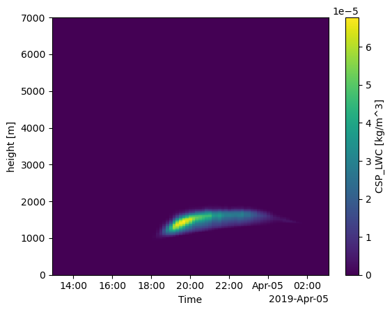
plot_thl = ds_stat['CSP_TH'].assign_coords(height = (ds_stat["CSP_Z"]))
plot_thl.isel(Time=slice(6,None)).plot(x = 'Time',y = 'height', ylim=[0,7000],vmin=298,vmax=320)
<matplotlib.collections.QuadMesh at 0x31a77fa10>
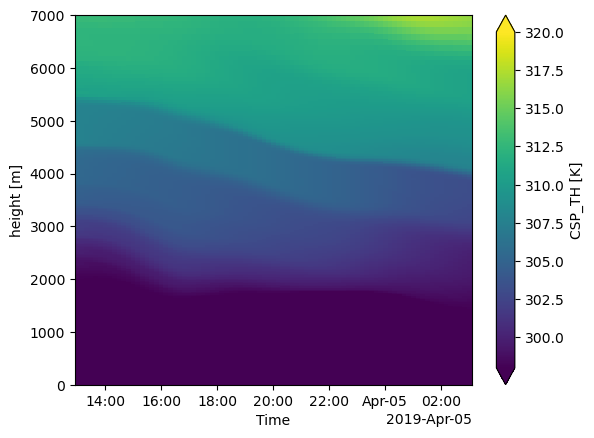
Fix some height things so that we can plot…
The z values are time dependent, so we need to deal with the height values by assuming that the first time step is close enough
We also need to make bottom_top a coordinate so that we aren’t yelled at by errors
ds_stat["bottom_top"] = ds_stat.bottom_top
ds_stat['bottom_top'] = ds_stat['CSP_Z'].isel(Time = 1).values
ds_stat['bottom_top'].values # make sure that these are heights and not indicies
array([   15.215184,    45.605114,    75.94632 ,   106.27506 ,
         136.59618 ,   166.91183 ,   197.23079 ,   227.55254 ,
         257.86115 ,   288.1541  ,   318.44684 ,   348.74237 ,
         379.03595 ,   409.33054 ,   439.62314 ,   469.91293 ,
         500.20493 ,   530.4964  ,   560.79016 ,   591.11    ,
         621.4132  ,   651.6837  ,   681.9462  ,   712.2066  ,
         742.4813  ,   772.7549  ,   803.0155  ,   833.27167 ,
         863.53253 ,   893.79333 ,   924.05646 ,   954.3343  ,
         984.625   ,  1014.9191  ,  1045.2263  ,  1075.5452  ,
        1105.8611  ,  1136.1669  ,  1166.4724  ,  1196.7739  ,
        1227.061   ,  1257.3391  ,  1287.613   ,  1317.8835  ,
        1348.1545  ,  1378.427   ,  1408.7014  ,  1438.9777  ,
        1469.2583  ,  1499.5316  ,  1529.7927  ,  1560.058   ,
        1590.3406  ,  1620.6185  ,  1650.8711  ,  1681.1194  ,
        1711.373   ,  1741.6282  ,  1771.863   ,  1802.084   ,
        1832.3059  ,  1862.5199  ,  1892.7288  ,  1922.9358  ,
        1953.1406  ,  1983.3519  ,  2013.5719  ,  2043.8057  ,
        2074.0422  ,  2104.2583  ,  2134.4634  ,  2164.6702  ,
        2194.8755  ,  2225.0752  ,  2255.268   ,  2285.4622  ,
        2315.6643  ,  2345.861   ,  2376.0405  ,  2406.2173  ,
        2436.3982  ,  2466.58    ,  2496.766   ,  2526.9626  ,
        2557.1538  ,  2587.3315  ,  2617.5088  ,  2647.6782  ,
        2677.8381  ,  2708.0024  ,  2738.185   ,  2768.3545  ,
        2798.5044  ,  2828.6675  ,  2858.8428  ,  2889.018   ,
        2919.1719  ,  2949.3062  ,  2979.443   ,  3009.5776  ,
        3039.703   ,  3069.83    ,  3099.9514  ,  3130.066   ,
        3160.1882  ,  3190.3154  ,  3220.4434  ,  3250.5742  ,
        3280.702   ,  3310.8237  ,  3340.931   ,  3371.0188  ,
        3401.102   ,  3431.1902  ,  3461.293   ,  3491.3945  ,
        3521.4683  ,  3551.5403  ,  3581.6167  ,  3611.6907  ,
        3641.769   ,  3671.8528  ,  3701.933   ,  3732.0137  ,
        3762.0945  ,  3792.1685  ,  3822.2473  ,  3852.3481  ,
        3882.4512  ,  3912.5269  ,  3942.5942  ,  3972.6646  ,
        4002.7378  ,  4032.811   ,  4062.8813  ,  4092.9517  ,
        4123.02    ,  4153.09    ,  4183.161   ,  4213.229   ,
        4243.2993  ,  4273.3696  ,  4303.4385  ,  4333.5093  ,
        4363.5786  ,  4393.6553  ,  4423.735   ,  4453.8096  ,
        4483.88    ,  4513.9585  ,  4544.05    ,  4574.1533  ,
        4604.2773  ,  4634.3887  ,  4664.45    ,  4694.4854  ,
        4724.5103  ,  4754.531   ,  4784.547   ,  4814.564   ,
        4844.583   ,  4874.598   ,  4904.608   ,  4934.618   ,
        4964.6323  ,  4994.6475  ,  5024.664   ,  5055.481   ,
        5087.9473  ,  5122.214   ,  5158.3315  ,  5196.3467  ,
        5236.46    ,  5278.7236  ,  5323.2344  ,  5370.1943  ,
        5419.6626  ,  5471.841   ,  5526.9717  ,  5585.007   ,
        5646.068   ,  5710.3896  ,  5778.146   ,  5849.596   ,
        5924.9067  ,  6004.247   ,  6087.865   ,  6176.043   ,
        6268.9814  ,  6366.915   ,  6470.13    ,  6578.867   ,
        6693.4404  ,  6814.2485  ,  6941.7056  ,  7076.026   ,
        7217.5884  ,  7366.8086  ,  7524.0337  ,  7689.741   ,
        7864.397   ,  8048.4517  ,  8242.3955  ,  8446.839   ,
        8662.638   ,  8890.157   ,  9130.356   ,  9383.886   ,
        9650.805   ,  9932.354   , 10227.337   , 10527.948   ,
       10828.727   , 11129.923   , 11431.03    , 11731.875   ,
       12032.737   , 12333.832   , 12635.557   , 12937.003   ,
       13237.864   , 13538.295   , 13838.356   , 14138.922   ,
       14440.3545  , 14719.19    ], dtype=float32)
Calculate cloud base and top from the liquid water conent and the liquid water mixing ratio
ds_stat['cb_lwc'] = (ds_stat['CSP_LWC']>0).idxmax(dim = 'bottom_top')
ds_stat['cb_lwc'] = ds_stat['cb_lwc'].where(ds_stat['cb_lwc']>ds_stat['bottom_top'][0])
print(ds_stat['cb_lwc'])

ds_stat['ct_lwc'] = ((ds_stat['CSP_LWC'].isel(bottom_top = slice(None, None, -1)))>0).idxmax(dim='bottom_top')
ds_stat['ct_lwc'] = ds_stat['ct_lwc'].where(ds_stat['ct_lwc']<ds_stat['bottom_top'][-1])
print(ds_stat['ct_lwc'])
<xarray.DataArray 'cb_lwc' (Time: 91)> Size: 364B
dask.array<where, shape=(91,), dtype=float32, chunksize=(1,), chunktype=numpy.ndarray>
Coordinates:
    XTIME    (Time) datetime64[ns] 728B dask.array<chunksize=(91,), meta=np.ndarray>
  * Time     (Time) datetime64[ns] 728B 2019-04-04T12:00:00 ... 2019-04-05T03...
<xarray.DataArray 'ct_lwc' (Time: 91)> Size: 364B
dask.array<where, shape=(91,), dtype=float32, chunksize=(1,), chunktype=numpy.ndarray>
Coordinates:
    XTIME    (Time) datetime64[ns] 728B dask.array<chunksize=(91,), meta=np.ndarray>
  * Time     (Time) datetime64[ns] 728B 2019-04-04T12:00:00 ... 2019-04-05T03...
ds_stat['cb_lwc'].plot(label='base',ylim = (0,7000),xlim = (ds_stat['CSP_Z'].Time[6],ds_stat['CSP_Z'].Time[-1]))
ds_stat['ct_lwc'].plot(label='top',ylim = (0,7000),xlim = (ds_stat['CSP_Z'].Time[6],ds_stat['CSP_Z'].Time[-1]))
plt.legend()
plt.ylabel('Height (m)')
plt.xlabel('Time (UTC)')
plt.show()
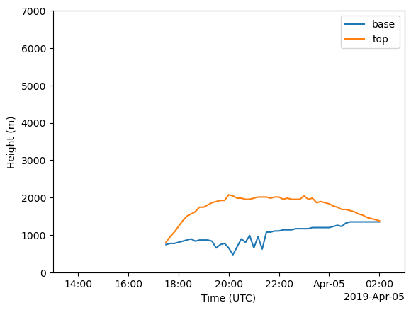
ds_stat['cb_ql'] = (ds_stat['CSP_LWC']>0).idxmax(dim = 'bottom_top')
ds_stat['cb_ql'] = ds_stat['cb_ql'].where(ds_stat['cb_ql']>ds_stat['bottom_top'][0])
print(ds_stat['cb_ql'].load())

ds_stat['ct_ql'] = ((ds_stat['CSP_LWC'].isel(bottom_top = slice(None, None, -1)))>0).idxmax(dim='bottom_top')
ds_stat['ct_ql'] = ds_stat['ct_ql'].where(ds_stat['ct_ql']<ds_stat['bottom_top'][-1])
print(ds_stat['ct_ql'].load())
<xarray.DataArray 'cb_ql' (Time: 91)> Size: 364B
array([       nan,        nan,        nan,        nan,        nan,
              nan,        nan,        nan,        nan,        nan,
              nan,        nan,        nan,        nan,        nan,
              nan,        nan,        nan,        nan,        nan,
              nan,        nan,        nan,        nan,        nan,
              nan,        nan,        nan,        nan,        nan,
              nan,        nan,        nan,  742.4813 ,  772.7549 ,
        772.7549 ,  803.0155 ,  833.27167,  863.53253,  893.79333,
        833.27167,  863.53253,  863.53253,  863.53253,  833.27167,
        651.6837 ,  742.4813 ,  772.7549 ,  651.6837 ,  469.91293,
        681.9462 ,  893.79333,  803.0155 ,  984.625  ,  651.6837 ,
        954.3343 ,  621.4132 , 1075.5452 , 1075.5452 , 1105.8611 ,
       1105.8611 , 1136.1669 , 1136.1669 , 1136.1669 , 1166.4724 ,
       1166.4724 , 1166.4724 , 1166.4724 , 1196.7739 , 1196.7739 ,
       1196.7739 , 1196.7739 , 1196.7739 , 1227.061  , 1257.3391 ,
       1227.061  , 1317.8835 , 1348.1545 , 1348.1545 , 1348.1545 ,
       1348.1545 , 1348.1545 , 1348.1545 , 1348.1545 , 1348.1545 ,
              nan,        nan,        nan,        nan,        nan,
              nan], dtype=float32)
Coordinates:
    XTIME    (Time) datetime64[ns] 728B 2019-04-04T12:00:00 ... 2019-04-05T03...
  * Time     (Time) datetime64[ns] 728B 2019-04-04T12:00:00 ... 2019-04-05T03...
<xarray.DataArray 'ct_ql' (Time: 91)> Size: 364B
array([      nan,       nan,       nan,       nan,       nan,       nan,
             nan,       nan,       nan,       nan,       nan,       nan,
             nan,       nan,       nan,       nan,       nan,       nan,
             nan,       nan,       nan,       nan,       nan,       nan,
             nan,       nan,       nan,       nan,       nan,       nan,
             nan,       nan,       nan,  803.0155,  954.3343, 1075.5452,
       1227.061 , 1378.427 , 1499.5316, 1560.058 , 1620.6185, 1741.6282,
       1741.6282, 1802.084 , 1862.5199, 1892.7288, 1922.9358, 1922.9358,
       2074.0422, 2043.8057, 1983.3519, 1983.3519, 1953.1406, 1953.1406,
       1983.3519, 2013.5719, 2013.5719, 2013.5719, 1983.3519, 2013.5719,
       2013.5719, 1953.1406, 1983.3519, 1953.1406, 1953.1406, 1953.1406,
       2043.8057, 1953.1406, 1983.3519, 1862.5199, 1892.7288, 1862.5199,
       1832.3059, 1771.863 , 1741.6282, 1681.1194, 1681.1194, 1650.8711,
       1620.6185, 1560.058 , 1529.7927, 1469.2583, 1438.9777, 1408.7014,
       1378.427 ,       nan,       nan,       nan,       nan,       nan,
             nan], dtype=float32)
Coordinates:
    XTIME    (Time) datetime64[ns] 728B 2019-04-04T12:00:00 ... 2019-04-05T03...
  * Time     (Time) datetime64[ns] 728B 2019-04-04T12:00:00 ... 2019-04-05T03...
ds_stat['cb_ql'].plot(label='base',ylim = (0,7000),xlim = (ds_stat['CSP_Z'].Time[6],ds_stat['CSP_Z'].Time[-1]))
ds_stat['ct_ql'].plot(label='top',ylim = (0,7000),xlim = (ds_stat['CSP_Z'].Time[6],ds_stat['CSP_Z'].Time[-1]))
plt.legend()
plt.ylabel('Height (m)')
plt.xlabel('Time (UTC)')
plt.show()
Conclusions
We notice how similar the cloud base/top are at their beginning and end times! This framework enables a streamlined method of analyzing clouds within the simulation data, including derived quantities such as cloud base/height.