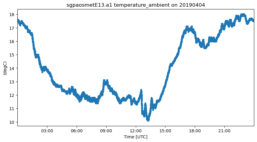
Simulation vs Observational Data of Shallow Cumulus Clouds over the Southern Great Plains on April 4th, 2019
Import
# Lasso Simulation Data

# import dask
from datetime import datetime
from distributed import Client
import numpy as np
import xarray as xr
import xwrf
import s3fs
import fsspec
import xarray as xr
import glob

import matplotlib.pyplot as plt
Spin up a Dask Cluster
We will use Dask here to access the data in a parallel/distributed manner.
client = Client()
client
/Users/mgrover/mambaforge/envs/lasso-those-clouds-cookbook-dev/lib/python3.12/site-packages/distributed/node.py:182: UserWarning: Port 8787 is already in use.
Perhaps you already have a cluster running?
Hosting the HTTP server on port 65202 instead
  warnings.warn(
Client
Client-9280965e-2a6e-11ef-a3bb-520a01803a93
| Connection method: Cluster object | Cluster type: distributed.LocalCluster |
| Dashboard: http://127.0.0.1:65202/status |
Cluster Info
LocalCluster
fb70a73c
| Dashboard: http://127.0.0.1:65202/status | Workers: 5 |
| Total threads: 10 | Total memory: 32.00 GiB |
| Status: running | Using processes: True |
Scheduler Info
Scheduler
Scheduler-8de6690b-bd21-465e-8d01-5fce5f777a90
| Comm: tcp://127.0.0.1:65203 | Workers: 5 |
| Dashboard: http://127.0.0.1:65202/status | Total threads: 10 |
| Started: Just now | Total memory: 32.00 GiB |
Workers
Worker: 0
| Comm: tcp://127.0.0.1:65216 | Total threads: 2 |
| Dashboard: http://127.0.0.1:65218/status | Memory: 6.40 GiB |
| Nanny: tcp://127.0.0.1:65206 | |
| Local directory: /var/folders/bw/c9j8z20x45s2y20vv6528qjc0000gq/T/dask-scratch-space/worker-ad8rksl2 | |
Worker: 1
| Comm: tcp://127.0.0.1:65222 | Total threads: 2 |
| Dashboard: http://127.0.0.1:65223/status | Memory: 6.40 GiB |
| Nanny: tcp://127.0.0.1:65208 | |
| Local directory: /var/folders/bw/c9j8z20x45s2y20vv6528qjc0000gq/T/dask-scratch-space/worker-h7ah2945 | |
Worker: 2
| Comm: tcp://127.0.0.1:65217 | Total threads: 2 |
| Dashboard: http://127.0.0.1:65219/status | Memory: 6.40 GiB |
| Nanny: tcp://127.0.0.1:65210 | |
| Local directory: /var/folders/bw/c9j8z20x45s2y20vv6528qjc0000gq/T/dask-scratch-space/worker-qqzdw3m1 | |
Worker: 3
| Comm: tcp://127.0.0.1:65225 | Total threads: 2 |
| Dashboard: http://127.0.0.1:65227/status | Memory: 6.40 GiB |
| Nanny: tcp://127.0.0.1:65212 | |
| Local directory: /var/folders/bw/c9j8z20x45s2y20vv6528qjc0000gq/T/dask-scratch-space/worker-e3ms7ha5 | |
Worker: 4
| Comm: tcp://127.0.0.1:65226 | Total threads: 2 |
| Dashboard: http://127.0.0.1:65229/status | Memory: 6.40 GiB |
| Nanny: tcp://127.0.0.1:65214 | |
| Local directory: /var/folders/bw/c9j8z20x45s2y20vv6528qjc0000gq/T/dask-scratch-space/worker-btowf9po | |
Access LASSO SGP Data from the NSF Jetstream Cloud
A subset of the LASSO Shallow Cumulus Experiment over the Southern Great Plains site has been made available on a cloud bucket, hosted through Project Pythia. These datasets were originally accessed through the LASSO bundle browser, untarred, then uploaded to the cloud bucket. We focus exclusively on the April 4, 2019 case.
Data were obtained from the Atmospheric Radiation Measurement (ARM) Program sponsored by the U.S. Department of Energy, Office of Science, Office of Biological and Environmental Research, Climate and Environmental Sciences Division.
Set the URL to access the data
The data are stored on a bucket, which is a web-accessible place where we can remotely stream the data, without downloading directly. The bucket is located on the NSF jetstream cloud, which we can see below. We then use fsspec to easily list the directrories and load in the data.
Below we set the url, then list (glob) the directories in the bucket.
# Set the URL and path for the cloud
URL = 'https://js2.jetstream-cloud.org:8001/'
path = f'pythia/lasso-sgp'


fs = fsspec.filesystem("s3", anon=True, client_kwargs=dict(endpoint_url=URL))

fs.glob(f"{path}/*")
['pythia/lasso-sgp/high_res_obs',
 'pythia/lasso-sgp/metrics',
 'pythia/lasso-sgp/sim0001',
 'pythia/lasso-sgp/sim0002',
 'pythia/lasso-sgp/sim0003',
 'pythia/lasso-sgp/sim0004',
 'pythia/lasso-sgp/sim0005',
 'pythia/lasso-sgp/sim0006',
 'pythia/lasso-sgp/sim0007',
 'pythia/lasso-sgp/sim0008']
We notice that there are 8 simulations, as well as observations in the bucket. We are going to start with the fourth simulation, setting a path to the actual output, which is under /raw_model/
case_date = datetime(2019, 4, 4)
sim_id = 4

# Read the wrfstat files
wrfstat_pattern = f's3://{path}/sim000{sim_id}/raw_model/wrfstat*'

# Read the wrfout files
wrfout_pattern = f's3://{path}/sim000{sim_id}/raw_model/wrfout*'

wrfstat_files = sorted(fs.glob(wrfstat_pattern))
wrfout_files = sorted(fs.glob(wrfout_pattern))
Now that we have lists of files, we setup a path to read into xarray since we need the bucket information as well.
wrfstat_file_list = [fs.open(file) for file in wrfstat_files]
wrfout_file_list = [fs.open(file) for file in wrfout_files]
Load Data Using Xarray and View Variables
We have a single WRF stat file, which we can load into xarray, then postprocess with xwrf.
ds_stat = xr.open_mfdataset(wrfstat_file_list, engine='h5netcdf').xwrf.postprocess()
ds_stat
<xarray.Dataset> Size: 72GB
Dimensions:         (Time: 91, z: 226, z_stag: 227, y: 250, x: 250,
                     x_stag: 251, y_stag: 251)
Coordinates:
    XTIME           (Time) datetime64[ns] 728B dask.array<chunksize=(91,), meta=np.ndarray>
  * Time            (Time) datetime64[ns] 728B 2019-04-04T12:00:00 ... 2019-0...
  * x_stag          (x_stag) float64 2kB -1.25e+04 -1.24e+04 ... 1.25e+04
  * x               (x) float64 2kB -1.245e+04 -1.235e+04 ... 1.245e+04
  * y               (y) float64 2kB -1.245e+04 -1.235e+04 ... 1.245e+04
  * y_stag          (y_stag) float64 2kB -1.25e+04 -1.24e+04 ... 1.25e+04
Dimensions without coordinates: z, z_stag
Data variables: (12/179)
    Times           (Time) |S19 2kB dask.array<chunksize=(1,), meta=np.ndarray>
    CST_CLDLOW      (Time) float32 364B dask.array<chunksize=(91,), meta=np.ndarray>
    CST_CLDTOT      (Time) float32 364B dask.array<chunksize=(91,), meta=np.ndarray>
    CST_LWP         (Time) float32 364B dask.array<chunksize=(91,), meta=np.ndarray>
    CST_IWP         (Time) float32 364B dask.array<chunksize=(91,), meta=np.ndarray>
    CST_PRECW       (Time) float32 364B dask.array<chunksize=(91,), meta=np.ndarray>
    ...              ...
    CSV_IWC         (Time, z, y, x) float32 5GB dask.array<chunksize=(1, 226, 125, 125), meta=np.ndarray>
    CSV_CLDFRAC     (Time, z, y, x) float32 5GB dask.array<chunksize=(1, 226, 125, 125), meta=np.ndarray>
    CSS_LWP         (Time, y, x) float32 23MB dask.array<chunksize=(1, 125, 125), meta=np.ndarray>
    CSS_IWP         (Time, y, x) float32 23MB dask.array<chunksize=(1, 125, 125), meta=np.ndarray>
    CSS_CLDTOT      (Time, y, x) float32 23MB dask.array<chunksize=(1, 125, 125), meta=np.ndarray>
    CSS_CLDLOW      (Time, y, x) float32 23MB dask.array<chunksize=(1, 125, 125), meta=np.ndarray>
Attributes: (12/96)
    TITLE:                                  OUTPUT FROM WRF V3.8.1 MODEL
    START_DATE:                            2019-04-04_12:00:00
    WEST-EAST_GRID_DIMENSION:              251
    SOUTH-NORTH_GRID_DIMENSION:            251
    BOTTOM-TOP_GRID_DIMENSION:             227
    DX:                                    100.0
    ...                                    ...
    config_aerosol:                        NA
    config_forecast_time:                  15.0 h
    config_boundary_method:                Periodic
    config_microphysics:                   Thompson (mp_physics=8)
    config_nickname:                       runlas20190404v1addhm
simulation_origin_host: cumulus-login2.ccs.ornl.gov- Time: 91
- z: 226
- z_stag: 227
- y: 250
- x: 250
- x_stag: 251
- y_stag: 251
- XTIME(Time)datetime64[ns]dask.array<chunksize=(91,), meta=np.ndarray>
- FieldType :
- 104
- MemoryOrder :
- 0
- description :
- minutes since 2019-04-04 12:00:00
- stagger :
Array Chunk Bytes 728 B 728 B Shape (91,) (91,) Dask graph 1 chunks in 2 graph layers Data type datetime64[ns] numpy.ndarray - Time(Time)datetime64[ns]2019-04-04T12:00:00 ... 2019-04-...
- long_name :
- Time
- standard_name :
- time
array(['2019-04-04T12:00:00.000000000', '2019-04-04T12:10:00.000000000', '2019-04-04T12:20:00.000000000', '2019-04-04T12:30:00.000000000', '2019-04-04T12:40:00.000000000', '2019-04-04T12:50:00.000000000', '2019-04-04T13:00:00.000000000', '2019-04-04T13:10:00.000000000', '2019-04-04T13:20:00.000000000', '2019-04-04T13:30:00.000000000', '2019-04-04T13:40:00.000000000', '2019-04-04T13:50:00.000000000', '2019-04-04T14:00:00.000000000', '2019-04-04T14:10:00.000000000', '2019-04-04T14:20:00.000000000', '2019-04-04T14:30:00.000000000', '2019-04-04T14:40:00.000000000', '2019-04-04T14:50:00.000000000', '2019-04-04T15:00:00.000000000', '2019-04-04T15:10:00.000000000', '2019-04-04T15:20:00.000000000', '2019-04-04T15:30:00.000000000', '2019-04-04T15:40:00.000000000', '2019-04-04T15:50:00.000000000', '2019-04-04T16:00:00.000000000', '2019-04-04T16:10:00.000000000', '2019-04-04T16:20:00.000000000', '2019-04-04T16:30:00.000000000', '2019-04-04T16:40:00.000000000', '2019-04-04T16:50:00.000000000', '2019-04-04T17:00:00.000000000', '2019-04-04T17:10:00.000000000', '2019-04-04T17:20:00.000000000', '2019-04-04T17:30:00.000000000', '2019-04-04T17:40:00.000000000', '2019-04-04T17:50:00.000000000', '2019-04-04T18:00:00.000000000', '2019-04-04T18:10:00.000000000', '2019-04-04T18:20:00.000000000', '2019-04-04T18:30:00.000000000', '2019-04-04T18:40:00.000000000', '2019-04-04T18:50:00.000000000', '2019-04-04T19:00:00.000000000', '2019-04-04T19:10:00.000000000', '2019-04-04T19:20:00.000000000', '2019-04-04T19:30:00.000000000', '2019-04-04T19:40:00.000000000', '2019-04-04T19:50:00.000000000', '2019-04-04T20:00:00.000000000', '2019-04-04T20:10:00.000000000', '2019-04-04T20:20:00.000000000', '2019-04-04T20:30:00.000000000', '2019-04-04T20:40:00.000000000', '2019-04-04T20:50:00.000000000', '2019-04-04T21:00:00.000000000', '2019-04-04T21:10:00.000000000', '2019-04-04T21:20:00.000000000', '2019-04-04T21:30:00.000000000', '2019-04-04T21:40:00.000000000', '2019-04-04T21:50:00.000000000', '2019-04-04T22:00:00.000000000', '2019-04-04T22:10:00.000000000', '2019-04-04T22:20:00.000000000', '2019-04-04T22:30:00.000000000', '2019-04-04T22:40:00.000000000', '2019-04-04T22:50:00.000000000', '2019-04-04T23:00:00.000000000', '2019-04-04T23:10:00.000000000', '2019-04-04T23:20:00.000000000', '2019-04-04T23:30:00.000000000', '2019-04-04T23:40:00.000000000', '2019-04-04T23:50:00.000000000', '2019-04-05T00:00:00.000000000', '2019-04-05T00:10:00.000000000', '2019-04-05T00:20:00.000000000', '2019-04-05T00:30:00.000000000', '2019-04-05T00:40:00.000000000', '2019-04-05T00:50:00.000000000', '2019-04-05T01:00:00.000000000', '2019-04-05T01:10:00.000000000', '2019-04-05T01:20:00.000000000', '2019-04-05T01:30:00.000000000', '2019-04-05T01:40:00.000000000', '2019-04-05T01:50:00.000000000', '2019-04-05T02:00:00.000000000', '2019-04-05T02:10:00.000000000', '2019-04-05T02:20:00.000000000', '2019-04-05T02:30:00.000000000', '2019-04-05T02:40:00.000000000', '2019-04-05T02:50:00.000000000', '2019-04-05T03:00:00.000000000'], dtype='datetime64[ns]') - x_stag(x_stag)float64-1.25e+04 -1.24e+04 ... 1.25e+04
- units :
- m
- standard_name :
- projection_x_coordinate
- axis :
- X
- c_grid_axis_shift :
- 0.5
array([-12500., -12400., -12300., ..., 12300., 12400., 12500.])
- x(x)float64-1.245e+04 -1.235e+04 ... 1.245e+04
- units :
- m
- standard_name :
- projection_x_coordinate
- axis :
- X
array([-12450., -12350., -12250., ..., 12250., 12350., 12450.])
- y(y)float64-1.245e+04 -1.235e+04 ... 1.245e+04
- units :
- m
- standard_name :
- projection_y_coordinate
- axis :
- Y
array([-12450., -12350., -12250., ..., 12250., 12350., 12450.])
- y_stag(y_stag)float64-1.25e+04 -1.24e+04 ... 1.25e+04
- units :
- m
- standard_name :
- projection_y_coordinate
- axis :
- Y
- c_grid_axis_shift :
- 0.5
array([-12500., -12400., -12300., ..., 12300., 12400., 12500.])
- Times(Time)|S19dask.array<chunksize=(1,), meta=np.ndarray>
Array Chunk Bytes 1.69 kiB 19 B Shape (91,) (1,) Dask graph 91 chunks in 2 graph layers Data type |S19 numpy.ndarray - CST_CLDLOW(Time)float32dask.array<chunksize=(91,), meta=np.ndarray>
- FieldType :
- 104
- MemoryOrder :
- 0
- description :
- Fractional low-cloud cover (<5 km)
- units :
- (0-1)
- stagger :
Array Chunk Bytes 364 B 364 B Shape (91,) (91,) Dask graph 1 chunks in 2 graph layers Data type float32 numpy.ndarray - CST_CLDTOT(Time)float32dask.array<chunksize=(91,), meta=np.ndarray>
- FieldType :
- 104
- MemoryOrder :
- 0
- description :
- Fractional cloud cover
- units :
- (0-1)
- stagger :
Array Chunk Bytes 364 B 364 B Shape (91,) (91,) Dask graph 1 chunks in 2 graph layers Data type float32 numpy.ndarray - CST_LWP(Time)float32dask.array<chunksize=(91,), meta=np.ndarray>
- FieldType :
- 104
- MemoryOrder :
- 0
- description :
- Vertical integrated liquid water path (based on ql)
- units :
- kg/m^2
- stagger :
Array Chunk Bytes 364 B 364 B Shape (91,) (91,) Dask graph 1 chunks in 2 graph layers Data type float32 numpy.ndarray - CST_IWP(Time)float32dask.array<chunksize=(91,), meta=np.ndarray>
- FieldType :
- 104
- MemoryOrder :
- 0
- description :
- Vertical integrated ice water path (based on qf)
- units :
- kg/m^2
- stagger :
Array Chunk Bytes 364 B 364 B Shape (91,) (91,) Dask graph 1 chunks in 2 graph layers Data type float32 numpy.ndarray - CST_PRECW(Time)float32dask.array<chunksize=(91,), meta=np.ndarray>
- FieldType :
- 104
- MemoryOrder :
- 0
- description :
- Vertical integrated water vapor
- units :
- kg/m^2
- stagger :
Array Chunk Bytes 364 B 364 B Shape (91,) (91,) Dask graph 1 chunks in 2 graph layers Data type float32 numpy.ndarray - CST_TKE(Time)float32dask.array<chunksize=(91,), meta=np.ndarray>
- FieldType :
- 104
- MemoryOrder :
- 0
- description :
- Vertical integrated TKE
- units :
- kg/s^2
- stagger :
Array Chunk Bytes 364 B 364 B Shape (91,) (91,) Dask graph 1 chunks in 2 graph layers Data type float32 numpy.ndarray - CST_TSAIR(Time)float32dask.array<chunksize=(91,), meta=np.ndarray>
- FieldType :
- 104
- MemoryOrder :
- 0
- description :
- Surface air temperature
- units :
- K
- stagger :
Array Chunk Bytes 364 B 364 B Shape (91,) (91,) Dask graph 1 chunks in 2 graph layers Data type float32 numpy.ndarray - CST_PS(Time)float32dask.array<chunksize=(91,), meta=np.ndarray>
- FieldType :
- 104
- MemoryOrder :
- 0
- description :
- Surface pressure
- units :
- Pa
- stagger :
Array Chunk Bytes 364 B 364 B Shape (91,) (91,) Dask graph 1 chunks in 2 graph layers Data type float32 numpy.ndarray - CST_PRECT(Time)float32dask.array<chunksize=(91,), meta=np.ndarray>
- FieldType :
- 104
- MemoryOrder :
- 0
- description :
- Total precipitation at surface
- units :
- mm/sec
- stagger :
Array Chunk Bytes 364 B 364 B Shape (91,) (91,) Dask graph 1 chunks in 2 graph layers Data type float32 numpy.ndarray - CST_SH(Time)float32dask.array<chunksize=(91,), meta=np.ndarray>
- FieldType :
- 104
- MemoryOrder :
- 0
- description :
- Surface sensible heat flux
- units :
- W/m^2
- stagger :
Array Chunk Bytes 364 B 364 B Shape (91,) (91,) Dask graph 1 chunks in 2 graph layers Data type float32 numpy.ndarray - CST_LH(Time)float32dask.array<chunksize=(91,), meta=np.ndarray>
- FieldType :
- 104
- MemoryOrder :
- 0
- description :
- Surface latent heat flux
- units :
- W/m^2
- stagger :
Array Chunk Bytes 364 B 364 B Shape (91,) (91,) Dask graph 1 chunks in 2 graph layers Data type float32 numpy.ndarray - CST_FSNTC(Time)float32dask.array<chunksize=(91,), meta=np.ndarray>
- FieldType :
- 104
- MemoryOrder :
- 0
- description :
- TOA SW net upward clear-sky radiation
- units :
- W/m^2
- stagger :
Array Chunk Bytes 364 B 364 B Shape (91,) (91,) Dask graph 1 chunks in 2 graph layers Data type float32 numpy.ndarray - CST_FSNT(Time)float32dask.array<chunksize=(91,), meta=np.ndarray>
- FieldType :
- 104
- MemoryOrder :
- 0
- description :
- TOA SW net upward total-sky radiation
- units :
- W/m^2
- stagger :
Array Chunk Bytes 364 B 364 B Shape (91,) (91,) Dask graph 1 chunks in 2 graph layers Data type float32 numpy.ndarray - CST_FLNTC(Time)float32dask.array<chunksize=(91,), meta=np.ndarray>
- FieldType :
- 104
- MemoryOrder :
- 0
- description :
- TOA LW (net) upward clear-sky radiation
- units :
- W/m^2
- stagger :
Array Chunk Bytes 364 B 364 B Shape (91,) (91,) Dask graph 1 chunks in 2 graph layers Data type float32 numpy.ndarray - CST_FLNT(Time)float32dask.array<chunksize=(91,), meta=np.ndarray>
- FieldType :
- 104
- MemoryOrder :
- 0
- description :
- TOA LW (net) upward total-sky radiation
- units :
- W/m^2
- stagger :
Array Chunk Bytes 364 B 364 B Shape (91,) (91,) Dask graph 1 chunks in 2 graph layers Data type float32 numpy.ndarray - CST_FSNSC(Time)float32dask.array<chunksize=(91,), meta=np.ndarray>
- FieldType :
- 104
- MemoryOrder :
- 0
- description :
- Surface SW net upward clear-sky radiation
- units :
- W/m^2
- stagger :
Array Chunk Bytes 364 B 364 B Shape (91,) (91,) Dask graph 1 chunks in 2 graph layers Data type float32 numpy.ndarray - CST_FSNS(Time)float32dask.array<chunksize=(91,), meta=np.ndarray>
- FieldType :
- 104
- MemoryOrder :
- 0
- description :
- Surface SW net upward total-sky radiation
- units :
- W/m^2
- stagger :
Array Chunk Bytes 364 B 364 B Shape (91,) (91,) Dask graph 1 chunks in 2 graph layers Data type float32 numpy.ndarray - CST_FLNSC(Time)float32dask.array<chunksize=(91,), meta=np.ndarray>
- FieldType :
- 104
- MemoryOrder :
- 0
- description :
- Surface LW net upward clear-sky radiation
- units :
- W/m^2
- stagger :
Array Chunk Bytes 364 B 364 B Shape (91,) (91,) Dask graph 1 chunks in 2 graph layers Data type float32 numpy.ndarray - CST_FLNS(Time)float32dask.array<chunksize=(91,), meta=np.ndarray>
- FieldType :
- 104
- MemoryOrder :
- 0
- description :
- Surface LW net upward total-sky radiation
- units :
- W/m^2
- stagger :
Array Chunk Bytes 364 B 364 B Shape (91,) (91,) Dask graph 1 chunks in 2 graph layers Data type float32 numpy.ndarray - CST_SWINC(Time)float32dask.array<chunksize=(91,), meta=np.ndarray>
- FieldType :
- 104
- MemoryOrder :
- 0
- description :
- TOA solar insolation
- units :
- W/m^2
- stagger :
Array Chunk Bytes 364 B 364 B Shape (91,) (91,) Dask graph 1 chunks in 2 graph layers Data type float32 numpy.ndarray - CST_TSK(Time)float32dask.array<chunksize=(91,), meta=np.ndarray>
- FieldType :
- 104
- MemoryOrder :
- 0
- description :
- Surface skin temperature
- units :
- K
- stagger :
Array Chunk Bytes 364 B 364 B Shape (91,) (91,) Dask graph 1 chunks in 2 graph layers Data type float32 numpy.ndarray - CST_UST(Time)float32dask.array<chunksize=(91,), meta=np.ndarray>
- FieldType :
- 104
- MemoryOrder :
- 0
- description :
- Surface friction velocity
- units :
- m/s
- stagger :
Array Chunk Bytes 364 B 364 B Shape (91,) (91,) Dask graph 1 chunks in 2 graph layers Data type float32 numpy.ndarray - CSP_Z(Time, z)float32dask.array<chunksize=(1, 226), meta=np.ndarray>
- FieldType :
- 104
- MemoryOrder :
- Z
- description :
- Half level height
- units :
- m
- stagger :
Array Chunk Bytes 80.34 kiB 904 B Shape (91, 226) (1, 226) Dask graph 91 chunks in 2 graph layers Data type float32 numpy.ndarray - CSP_Z8W(Time, z_stag)float32dask.array<chunksize=(1, 227), meta=np.ndarray>
- FieldType :
- 104
- MemoryOrder :
- Z
- description :
- Full level height
- units :
- m
- stagger :
- Z
Array Chunk Bytes 80.69 kiB 908 B Shape (91, 227) (1, 227) Dask graph 91 chunks in 2 graph layers Data type float32 numpy.ndarray - CSP_DZ8W(Time, z)float32dask.array<chunksize=(1, 226), meta=np.ndarray>
- FieldType :
- 104
- MemoryOrder :
- Z
- description :
- dz at full level
- units :
- m
- stagger :
Array Chunk Bytes 80.34 kiB 904 B Shape (91, 226) (1, 226) Dask graph 91 chunks in 2 graph layers Data type float32 numpy.ndarray - CSP_U(Time, z)float32dask.array<chunksize=(1, 226), meta=np.ndarray>
- FieldType :
- 104
- MemoryOrder :
- Z
- description :
- Zonal wind
- units :
- m/s
- stagger :
Array Chunk Bytes 80.34 kiB 904 B Shape (91, 226) (1, 226) Dask graph 91 chunks in 2 graph layers Data type float32 numpy.ndarray - CSP_V(Time, z)float32dask.array<chunksize=(1, 226), meta=np.ndarray>
- FieldType :
- 104
- MemoryOrder :
- Z
- description :
- Meridional wind
- units :
- m/s
- stagger :
Array Chunk Bytes 80.34 kiB 904 B Shape (91, 226) (1, 226) Dask graph 91 chunks in 2 graph layers Data type float32 numpy.ndarray - CSP_W(Time, z_stag)float32dask.array<chunksize=(1, 227), meta=np.ndarray>
- FieldType :
- 104
- MemoryOrder :
- Z
- description :
- Vertical motion
- units :
- m/s
- stagger :
- Z
Array Chunk Bytes 80.69 kiB 908 B Shape (91, 227) (1, 227) Dask graph 91 chunks in 2 graph layers Data type float32 numpy.ndarray - CSP_P(Time, z)float32dask.array<chunksize=(1, 226), meta=np.ndarray>
- FieldType :
- 104
- MemoryOrder :
- Z
- description :
- Pressure
- units :
- Pa
- stagger :
Array Chunk Bytes 80.34 kiB 904 B Shape (91, 226) (1, 226) Dask graph 91 chunks in 2 graph layers Data type float32 numpy.ndarray - CSP_TH(Time, z)float32dask.array<chunksize=(1, 226), meta=np.ndarray>
- FieldType :
- 104
- MemoryOrder :
- Z
- description :
- Potential temperature
- units :
- K
- stagger :
Array Chunk Bytes 80.34 kiB 904 B Shape (91, 226) (1, 226) Dask graph 91 chunks in 2 graph layers Data type float32 numpy.ndarray - CSP_THV(Time, z)float32dask.array<chunksize=(1, 226), meta=np.ndarray>
- FieldType :
- 104
- MemoryOrder :
- Z
- description :
- Virtual potential temperature
- units :
- K
- stagger :
Array Chunk Bytes 80.34 kiB 904 B Shape (91, 226) (1, 226) Dask graph 91 chunks in 2 graph layers Data type float32 numpy.ndarray - CSP_THL(Time, z)float32dask.array<chunksize=(1, 226), meta=np.ndarray>
- FieldType :
- 104
- MemoryOrder :
- Z
- description :
- Liquid water potential temperature
- units :
- K
- stagger :
Array Chunk Bytes 80.34 kiB 904 B Shape (91, 226) (1, 226) Dask graph 91 chunks in 2 graph layers Data type float32 numpy.ndarray - CSP_QV(Time, z)float32dask.array<chunksize=(1, 226), meta=np.ndarray>
- FieldType :
- 104
- MemoryOrder :
- Z
- description :
- Water vapor mixing ratio
- units :
- kg/kg
- stagger :
Array Chunk Bytes 80.34 kiB 904 B Shape (91, 226) (1, 226) Dask graph 91 chunks in 2 graph layers Data type float32 numpy.ndarray - CSP_QC(Time, z)float32dask.array<chunksize=(1, 226), meta=np.ndarray>
- FieldType :
- 104
- MemoryOrder :
- Z
- description :
- Cloud water mixing ratio
- units :
- kg/kg
- stagger :
Array Chunk Bytes 80.34 kiB 904 B Shape (91, 226) (1, 226) Dask graph 91 chunks in 2 graph layers Data type float32 numpy.ndarray - CSP_QI(Time, z)float32dask.array<chunksize=(1, 226), meta=np.ndarray>
- FieldType :
- 104
- MemoryOrder :
- Z
- description :
- Ice crystal (cloud ice) mixing ratio
- units :
- kg/kg
- stagger :
Array Chunk Bytes 80.34 kiB 904 B Shape (91, 226) (1, 226) Dask graph 91 chunks in 2 graph layers Data type float32 numpy.ndarray - CSP_QL(Time, z)float32dask.array<chunksize=(1, 226), meta=np.ndarray>
- FieldType :
- 104
- MemoryOrder :
- Z
- description :
- Liquid water mixing ratio
- units :
- kg/kg
- stagger :
Array Chunk Bytes 80.34 kiB 904 B Shape (91, 226) (1, 226) Dask graph 91 chunks in 2 graph layers Data type float32 numpy.ndarray - CSP_QF(Time, z)float32dask.array<chunksize=(1, 226), meta=np.ndarray>
- FieldType :
- 104
- MemoryOrder :
- Z
- description :
- Frozen water mixing ratio
- units :
- kg/kg
- stagger :
Array Chunk Bytes 80.34 kiB 904 B Shape (91, 226) (1, 226) Dask graph 91 chunks in 2 graph layers Data type float32 numpy.ndarray - CSP_QT(Time, z)float32dask.array<chunksize=(1, 226), meta=np.ndarray>
- FieldType :
- 104
- MemoryOrder :
- Z
- description :
- Total (vapor+liquid+frozen) water mixing ratio
- units :
- kg/kg
- stagger :
Array Chunk Bytes 80.34 kiB 904 B Shape (91, 226) (1, 226) Dask graph 91 chunks in 2 graph layers Data type float32 numpy.ndarray - CSP_LWC(Time, z)float32dask.array<chunksize=(1, 226), meta=np.ndarray>
- FieldType :
- 104
- MemoryOrder :
- Z
- description :
- Liquid water content (based on ql)
- units :
- kg/m^3
- stagger :
Array Chunk Bytes 80.34 kiB 904 B Shape (91, 226) (1, 226) Dask graph 91 chunks in 2 graph layers Data type float32 numpy.ndarray - CSP_IWC(Time, z)float32dask.array<chunksize=(1, 226), meta=np.ndarray>
- FieldType :
- 104
- MemoryOrder :
- Z
- description :
- Ice water content (based on qf)
- units :
- kg/m^3
- stagger :
Array Chunk Bytes 80.34 kiB 904 B Shape (91, 226) (1, 226) Dask graph 91 chunks in 2 graph layers Data type float32 numpy.ndarray - CSP_SPEQV(Time, z)float32dask.array<chunksize=(1, 226), meta=np.ndarray>
- FieldType :
- 104
- MemoryOrder :
- Z
- description :
- Specific humidity
- units :
- kg/kg
- stagger :
Array Chunk Bytes 80.34 kiB 904 B Shape (91, 226) (1, 226) Dask graph 91 chunks in 2 graph layers Data type float32 numpy.ndarray - CSP_A_CL(Time, z)float32dask.array<chunksize=(1, 226), meta=np.ndarray>
- FieldType :
- 104
- MemoryOrder :
- Z
- description :
- Fraction of cloudy grid points
- units :
- (0-1)
- stagger :
Array Chunk Bytes 80.34 kiB 904 B Shape (91, 226) (1, 226) Dask graph 91 chunks in 2 graph layers Data type float32 numpy.ndarray - CSP_RHO(Time, z)float32dask.array<chunksize=(1, 226), meta=np.ndarray>
- FieldType :
- 104
- MemoryOrder :
- Z
- description :
- Density
- units :
- kg/m^3
- stagger :
Array Chunk Bytes 80.34 kiB 904 B Shape (91, 226) (1, 226) Dask graph 91 chunks in 2 graph layers Data type float32 numpy.ndarray - CSP_U2(Time, z)float32dask.array<chunksize=(1, 226), meta=np.ndarray>
- FieldType :
- 104
- MemoryOrder :
- Z
- description :
- u_p^2
- units :
- m^2/s^2
- stagger :
Array Chunk Bytes 80.34 kiB 904 B Shape (91, 226) (1, 226) Dask graph 91 chunks in 2 graph layers Data type float32 numpy.ndarray - CSP_V2(Time, z)float32dask.array<chunksize=(1, 226), meta=np.ndarray>
- FieldType :
- 104
- MemoryOrder :
- Z
- description :
- v_p^2
- units :
- m^2/s^2
- stagger :
Array Chunk Bytes 80.34 kiB 904 B Shape (91, 226) (1, 226) Dask graph 91 chunks in 2 graph layers Data type float32 numpy.ndarray - CSP_U2V2(Time, z)float32dask.array<chunksize=(1, 226), meta=np.ndarray>
- FieldType :
- 104
- MemoryOrder :
- Z
- description :
- u_p^2+v_p^2
- units :
- m^2/s^2
- stagger :
Array Chunk Bytes 80.34 kiB 904 B Shape (91, 226) (1, 226) Dask graph 91 chunks in 2 graph layers Data type float32 numpy.ndarray - CSP_W2(Time, z_stag)float32dask.array<chunksize=(1, 227), meta=np.ndarray>
- FieldType :
- 104
- MemoryOrder :
- Z
- description :
- w_p^2
- units :
- m^2/s^2
- stagger :
- Z
Array Chunk Bytes 80.69 kiB 908 B Shape (91, 227) (1, 227) Dask graph 91 chunks in 2 graph layers Data type float32 numpy.ndarray - CSP_W3(Time, z_stag)float32dask.array<chunksize=(1, 227), meta=np.ndarray>
- FieldType :
- 104
- MemoryOrder :
- Z
- description :
- w_p^3
- units :
- m^3/s^3
- stagger :
- Z
Array Chunk Bytes 80.69 kiB 908 B Shape (91, 227) (1, 227) Dask graph 91 chunks in 2 graph layers Data type float32 numpy.ndarray - CSP_WSKEW(Time, z_stag)float32dask.array<chunksize=(1, 227), meta=np.ndarray>
- FieldType :
- 104
- MemoryOrder :
- Z
- description :
- Skewness <w3>/<w2>^(3/2)
- units :
- stagger :
- Z
Array Chunk Bytes 80.69 kiB 908 B Shape (91, 227) (1, 227) Dask graph 91 chunks in 2 graph layers Data type float32 numpy.ndarray - CSP_UW(Time, z)float32dask.array<chunksize=(1, 226), meta=np.ndarray>
- FieldType :
- 104
- MemoryOrder :
- Z
- description :
- x-momentum flux uw (rs+sgs)
- units :
- m^2/s^2
- stagger :
Array Chunk Bytes 80.34 kiB 904 B Shape (91, 226) (1, 226) Dask graph 91 chunks in 2 graph layers Data type float32 numpy.ndarray - CSP_VW(Time, z)float32dask.array<chunksize=(1, 226), meta=np.ndarray>
- FieldType :
- 104
- MemoryOrder :
- Z
- description :
- y-momentum flux vw (rs+sgs)
- units :
- m^2/s^2
- stagger :
Array Chunk Bytes 80.34 kiB 904 B Shape (91, 226) (1, 226) Dask graph 91 chunks in 2 graph layers Data type float32 numpy.ndarray - CSP_WTH(Time, z)float32dask.array<chunksize=(1, 226), meta=np.ndarray>
- FieldType :
- 104
- MemoryOrder :
- Z
- description :
- Potential temperature flux (rs+sgs)
- units :
- K m/s
- stagger :
Array Chunk Bytes 80.34 kiB 904 B Shape (91, 226) (1, 226) Dask graph 91 chunks in 2 graph layers Data type float32 numpy.ndarray - CSP_WTHV(Time, z)float32dask.array<chunksize=(1, 226), meta=np.ndarray>
- FieldType :
- 104
- MemoryOrder :
- Z
- description :
- Virtual potential temperature flux (rs+sgs)
- units :
- K m/s
- stagger :
Array Chunk Bytes 80.34 kiB 904 B Shape (91, 226) (1, 226) Dask graph 91 chunks in 2 graph layers Data type float32 numpy.ndarray - CSP_WTHL(Time, z)float32dask.array<chunksize=(1, 226), meta=np.ndarray>
- FieldType :
- 104
- MemoryOrder :
- Z
- description :
- Liquid water potential temperature flux (rs+sgs)
- units :
- K m/s
- stagger :
Array Chunk Bytes 80.34 kiB 904 B Shape (91, 226) (1, 226) Dask graph 91 chunks in 2 graph layers Data type float32 numpy.ndarray - CSP_WQV(Time, z)float32dask.array<chunksize=(1, 226), meta=np.ndarray>
- FieldType :
- 104
- MemoryOrder :
- Z
- description :
- Water vapor flux (rs+sgs)
- units :
- kg/kg m/s
- stagger :
Array Chunk Bytes 80.34 kiB 904 B Shape (91, 226) (1, 226) Dask graph 91 chunks in 2 graph layers Data type float32 numpy.ndarray - CSP_WQC(Time, z)float32dask.array<chunksize=(1, 226), meta=np.ndarray>
- FieldType :
- 104
- MemoryOrder :
- Z
- description :
- Cloud water flux (rs+sgs)
- units :
- kg/kg m/s
- stagger :
Array Chunk Bytes 80.34 kiB 904 B Shape (91, 226) (1, 226) Dask graph 91 chunks in 2 graph layers Data type float32 numpy.ndarray - CSP_WQI(Time, z)float32dask.array<chunksize=(1, 226), meta=np.ndarray>
- FieldType :
- 104
- MemoryOrder :
- Z
- description :
- Ice crystal (cloud ice) flux (rs+sgs)
- units :
- kg/kg m/s
- stagger :
Array Chunk Bytes 80.34 kiB 904 B Shape (91, 226) (1, 226) Dask graph 91 chunks in 2 graph layers Data type float32 numpy.ndarray - CSP_WQL(Time, z)float32dask.array<chunksize=(1, 226), meta=np.ndarray>
- FieldType :
- 104
- MemoryOrder :
- Z
- description :
- Liquid water flux (rs+sgs)
- units :
- kg/kg m/s
- stagger :
Array Chunk Bytes 80.34 kiB 904 B Shape (91, 226) (1, 226) Dask graph 91 chunks in 2 graph layers Data type float32 numpy.ndarray - CSP_WQF(Time, z)float32dask.array<chunksize=(1, 226), meta=np.ndarray>
- FieldType :
- 104
- MemoryOrder :
- Z
- description :
- Frozen water flux (rs+sgs)
- units :
- kg/kg m/s
- stagger :
Array Chunk Bytes 80.34 kiB 904 B Shape (91, 226) (1, 226) Dask graph 91 chunks in 2 graph layers Data type float32 numpy.ndarray - CSP_WQT(Time, z)float32dask.array<chunksize=(1, 226), meta=np.ndarray>
- FieldType :
- 104
- MemoryOrder :
- Z
- description :
- Total water flux (rs+sgs)
- units :
- kg/kg m/s
- stagger :
Array Chunk Bytes 80.34 kiB 904 B Shape (91, 226) (1, 226) Dask graph 91 chunks in 2 graph layers Data type float32 numpy.ndarray - CSP_UW_SGS(Time, z)float32dask.array<chunksize=(1, 226), meta=np.ndarray>
- FieldType :
- 104
- MemoryOrder :
- Z
- description :
- x-momentum flux uw (sgs)
- units :
- m^2/s^2
- stagger :
Array Chunk Bytes 80.34 kiB 904 B Shape (91, 226) (1, 226) Dask graph 91 chunks in 2 graph layers Data type float32 numpy.ndarray - CSP_VW_SGS(Time, z)float32dask.array<chunksize=(1, 226), meta=np.ndarray>
- FieldType :
- 104
- MemoryOrder :
- Z
- description :
- y-momentum flux vw (sgs)
- units :
- m^2/s^2
- stagger :
Array Chunk Bytes 80.34 kiB 904 B Shape (91, 226) (1, 226) Dask graph 91 chunks in 2 graph layers Data type float32 numpy.ndarray - CSP_WTH_SGS(Time, z)float32dask.array<chunksize=(1, 226), meta=np.ndarray>
- FieldType :
- 104
- MemoryOrder :
- Z
- description :
- Potential temperature flux (sgs)
- units :
- K m/s
- stagger :
Array Chunk Bytes 80.34 kiB 904 B Shape (91, 226) (1, 226) Dask graph 91 chunks in 2 graph layers Data type float32 numpy.ndarray - CSP_WTHV_SGS(Time, z)float32dask.array<chunksize=(1, 226), meta=np.ndarray>
- FieldType :
- 104
- MemoryOrder :
- Z
- description :
- Virtual potential temperature flux (sgs)
- units :
- K m/s
- stagger :
Array Chunk Bytes 80.34 kiB 904 B Shape (91, 226) (1, 226) Dask graph 91 chunks in 2 graph layers Data type float32 numpy.ndarray - CSP_WTHL_SGS(Time, z)float32dask.array<chunksize=(1, 226), meta=np.ndarray>
- FieldType :
- 104
- MemoryOrder :
- Z
- description :
- Liquid water potential temperature flux (sgs)
- units :
- K m/s
- stagger :
Array Chunk Bytes 80.34 kiB 904 B Shape (91, 226) (1, 226) Dask graph 91 chunks in 2 graph layers Data type float32 numpy.ndarray - CSP_WQV_SGS(Time, z)float32dask.array<chunksize=(1, 226), meta=np.ndarray>
- FieldType :
- 104
- MemoryOrder :
- Z
- description :
- Water vapor flux (sgs)
- units :
- kg/kg m/s
- stagger :
Array Chunk Bytes 80.34 kiB 904 B Shape (91, 226) (1, 226) Dask graph 91 chunks in 2 graph layers Data type float32 numpy.ndarray - CSP_WQC_SGS(Time, z)float32dask.array<chunksize=(1, 226), meta=np.ndarray>
- FieldType :
- 104
- MemoryOrder :
- Z
- description :
- Cloud water flux (sgs)
- units :
- kg/kg m/s
- stagger :
Array Chunk Bytes 80.34 kiB 904 B Shape (91, 226) (1, 226) Dask graph 91 chunks in 2 graph layers Data type float32 numpy.ndarray - CSP_WQI_SGS(Time, z)float32dask.array<chunksize=(1, 226), meta=np.ndarray>
- FieldType :
- 104
- MemoryOrder :
- Z
- description :
- Ice crystal (cloud ice) flux (sgs)
- units :
- kg/kg m/s
- stagger :
Array Chunk Bytes 80.34 kiB 904 B Shape (91, 226) (1, 226) Dask graph 91 chunks in 2 graph layers Data type float32 numpy.ndarray - CSP_WQL_SGS(Time, z)float32dask.array<chunksize=(1, 226), meta=np.ndarray>
- FieldType :
- 104
- MemoryOrder :
- Z
- description :
- Liquid water flux (sgs)
- units :
- kg/kg m/s
- stagger :
Array Chunk Bytes 80.34 kiB 904 B Shape (91, 226) (1, 226) Dask graph 91 chunks in 2 graph layers Data type float32 numpy.ndarray - CSP_WQF_SGS(Time, z)float32dask.array<chunksize=(1, 226), meta=np.ndarray>
- FieldType :
- 104
- MemoryOrder :
- Z
- description :
- Frozen water flux (sgs)
- units :
- kg/kg m/s
- stagger :
Array Chunk Bytes 80.34 kiB 904 B Shape (91, 226) (1, 226) Dask graph 91 chunks in 2 graph layers Data type float32 numpy.ndarray - CSP_WQT_SGS(Time, z)float32dask.array<chunksize=(1, 226), meta=np.ndarray>
- FieldType :
- 104
- MemoryOrder :
- Z
- description :
- Total water flux (sgs)
- units :
- kg/kg m/s
- stagger :
Array Chunk Bytes 80.34 kiB 904 B Shape (91, 226) (1, 226) Dask graph 91 chunks in 2 graph layers Data type float32 numpy.ndarray - CSP_SEDFQC(Time, z)float32dask.array<chunksize=(1, 226), meta=np.ndarray>
- FieldType :
- 104
- MemoryOrder :
- Z
- description :
- Sedimentation flux of qc
- units :
- kg /m^2/s
- stagger :
Array Chunk Bytes 80.34 kiB 904 B Shape (91, 226) (1, 226) Dask graph 91 chunks in 2 graph layers Data type float32 numpy.ndarray - CSP_SEDFQR(Time, z)float32dask.array<chunksize=(1, 226), meta=np.ndarray>
- FieldType :
- 104
- MemoryOrder :
- Z
- description :
- Sedimentation (Precipitation) flux of qr
- units :
- kg /m^2/s
- stagger :
Array Chunk Bytes 80.34 kiB 904 B Shape (91, 226) (1, 226) Dask graph 91 chunks in 2 graph layers Data type float32 numpy.ndarray - CSP_THDT_COND(Time, z)float32dask.array<chunksize=(1, 226), meta=np.ndarray>
- FieldType :
- 104
- MemoryOrder :
- Z
- description :
- dth/dt due to net condensation
- units :
- K/s
- stagger :
Array Chunk Bytes 80.34 kiB 904 B Shape (91, 226) (1, 226) Dask graph 91 chunks in 2 graph layers Data type float32 numpy.ndarray - CSP_THDT_LW(Time, z)float32dask.array<chunksize=(1, 226), meta=np.ndarray>
- FieldType :
- 104
- MemoryOrder :
- Z
- description :
- dth/dt due to LW radiation
- units :
- K/s
- stagger :
Array Chunk Bytes 80.34 kiB 904 B Shape (91, 226) (1, 226) Dask graph 91 chunks in 2 graph layers Data type float32 numpy.ndarray - CSP_THDT_SW(Time, z)float32dask.array<chunksize=(1, 226), meta=np.ndarray>
- FieldType :
- 104
- MemoryOrder :
- Z
- description :
- dth/dt due to SW radiation
- units :
- K/s
- stagger :
Array Chunk Bytes 80.34 kiB 904 B Shape (91, 226) (1, 226) Dask graph 91 chunks in 2 graph layers Data type float32 numpy.ndarray - CSP_THDT_LS(Time, z)float32dask.array<chunksize=(1, 226), meta=np.ndarray>
- FieldType :
- 104
- MemoryOrder :
- Z
- description :
- dth/dt due to large-scale forcing
- units :
- K/s
- stagger :
Array Chunk Bytes 80.34 kiB 904 B Shape (91, 226) (1, 226) Dask graph 91 chunks in 2 graph layers Data type float32 numpy.ndarray - CSP_QVDT_PR(Time, z)float32dask.array<chunksize=(1, 226), meta=np.ndarray>
- FieldType :
- 104
- MemoryOrder :
- Z
- description :
- dqv/dt due to conversion to precipitation
- units :
- kg/kg/s
- stagger :
Array Chunk Bytes 80.34 kiB 904 B Shape (91, 226) (1, 226) Dask graph 91 chunks in 2 graph layers Data type float32 numpy.ndarray - CSP_QVDT_COND(Time, z)float32dask.array<chunksize=(1, 226), meta=np.ndarray>
- FieldType :
- 104
- MemoryOrder :
- Z
- description :
- dqv/dt due to net condensation
- units :
- kg/kg/s
- stagger :
Array Chunk Bytes 80.34 kiB 904 B Shape (91, 226) (1, 226) Dask graph 91 chunks in 2 graph layers Data type float32 numpy.ndarray - CSP_QVDT_LS(Time, z)float32dask.array<chunksize=(1, 226), meta=np.ndarray>
- FieldType :
- 104
- MemoryOrder :
- Z
- description :
- dqv/dt due to large-scale forcing
- units :
- kg/kg/s
- stagger :
Array Chunk Bytes 80.34 kiB 904 B Shape (91, 226) (1, 226) Dask graph 91 chunks in 2 graph layers Data type float32 numpy.ndarray - CSP_QCDT_PR(Time, z)float32dask.array<chunksize=(1, 226), meta=np.ndarray>
- FieldType :
- 104
- MemoryOrder :
- Z
- description :
- dqc/dt due to conversion to precipitation
- units :
- kg/kg/s
- stagger :
Array Chunk Bytes 80.34 kiB 904 B Shape (91, 226) (1, 226) Dask graph 91 chunks in 2 graph layers Data type float32 numpy.ndarray - CSP_QCDT_SED(Time, z)float32dask.array<chunksize=(1, 226), meta=np.ndarray>
- FieldType :
- 104
- MemoryOrder :
- Z
- description :
- dqc/dt due to sedimentation
- units :
- kg/kg/s
- stagger :
Array Chunk Bytes 80.34 kiB 904 B Shape (91, 226) (1, 226) Dask graph 91 chunks in 2 graph layers Data type float32 numpy.ndarray - CSP_QRDT_SED(Time, z)float32dask.array<chunksize=(1, 226), meta=np.ndarray>
- FieldType :
- 104
- MemoryOrder :
- Z
- description :
- dqr/dt due to sedimentation
- units :
- kg/kg/s
- stagger :
Array Chunk Bytes 80.34 kiB 904 B Shape (91, 226) (1, 226) Dask graph 91 chunks in 2 graph layers Data type float32 numpy.ndarray - CSP_THDT_LSHOR(Time, z)float32dask.array<chunksize=(1, 226), meta=np.ndarray>
- FieldType :
- 104
- MemoryOrder :
- Z
- description :
- th tendency due to LS horizontal adv
- units :
- K s-1
- stagger :
Array Chunk Bytes 80.34 kiB 904 B Shape (91, 226) (1, 226) Dask graph 91 chunks in 2 graph layers Data type float32 numpy.ndarray - CSP_QVDT_LSHOR(Time, z)float32dask.array<chunksize=(1, 226), meta=np.ndarray>
- FieldType :
- 104
- MemoryOrder :
- Z
- description :
- qv tendency due to LS horizontal adv
- units :
- kg kg-1 s-1
- stagger :
Array Chunk Bytes 80.34 kiB 904 B Shape (91, 226) (1, 226) Dask graph 91 chunks in 2 graph layers Data type float32 numpy.ndarray - CSP_THDT_LSVER(Time, z)float32dask.array<chunksize=(1, 226), meta=np.ndarray>
- FieldType :
- 104
- MemoryOrder :
- Z
- description :
- th tendency due to LS horizontal adv
- units :
- K s-1
- stagger :
Array Chunk Bytes 80.34 kiB 904 B Shape (91, 226) (1, 226) Dask graph 91 chunks in 2 graph layers Data type float32 numpy.ndarray - CSP_QVDT_LSVER(Time, z)float32dask.array<chunksize=(1, 226), meta=np.ndarray>
- FieldType :
- 104
- MemoryOrder :
- Z
- description :
- qv tendency due to LS horizontal adv
- units :
- kg kg-1 s-1
- stagger :
Array Chunk Bytes 80.34 kiB 904 B Shape (91, 226) (1, 226) Dask graph 91 chunks in 2 graph layers Data type float32 numpy.ndarray - CSP_THDT_LSRLX(Time, z)float32dask.array<chunksize=(1, 226), meta=np.ndarray>
- FieldType :
- 104
- MemoryOrder :
- Z
- description :
- th tendency due to relaxation to LS
- units :
- K s-1
- stagger :
Array Chunk Bytes 80.34 kiB 904 B Shape (91, 226) (1, 226) Dask graph 91 chunks in 2 graph layers Data type float32 numpy.ndarray - CSP_QVDT_LSRLX(Time, z)float32dask.array<chunksize=(1, 226), meta=np.ndarray>
- FieldType :
- 104
- MemoryOrder :
- Z
- description :
- qv tendency due to relaxation to LS
- units :
- kg kg-1 s-1
- stagger :
Array Chunk Bytes 80.34 kiB 904 B Shape (91, 226) (1, 226) Dask graph 91 chunks in 2 graph layers Data type float32 numpy.ndarray - CSP_UDT_LS(Time, z)float32dask.array<chunksize=(1, 226), meta=np.ndarray>
- FieldType :
- 104
- MemoryOrder :
- Z
- description :
- u tendency due to LS forcing
- units :
- m s-2
- stagger :
Array Chunk Bytes 80.34 kiB 904 B Shape (91, 226) (1, 226) Dask graph 91 chunks in 2 graph layers Data type float32 numpy.ndarray - CSP_VDT_LS(Time, z)float32dask.array<chunksize=(1, 226), meta=np.ndarray>
- FieldType :
- 104
- MemoryOrder :
- Z
- description :
- v tendency due to LS forcing
- units :
- m s-2
- stagger :
Array Chunk Bytes 80.34 kiB 904 B Shape (91, 226) (1, 226) Dask graph 91 chunks in 2 graph layers Data type float32 numpy.ndarray - CSP_UDT_LSVER(Time, z)float32dask.array<chunksize=(1, 226), meta=np.ndarray>
- FieldType :
- 104
- MemoryOrder :
- Z
- description :
- u tendency due to LS vertical adv
- units :
- m s-2
- stagger :
Array Chunk Bytes 80.34 kiB 904 B Shape (91, 226) (1, 226) Dask graph 91 chunks in 2 graph layers Data type float32 numpy.ndarray - CSP_VDT_LSVER(Time, z)float32dask.array<chunksize=(1, 226), meta=np.ndarray>
- FieldType :
- 104
- MemoryOrder :
- Z
- description :
- v tendency due to LS vertical adv
- units :
- m s-2
- stagger :
Array Chunk Bytes 80.34 kiB 904 B Shape (91, 226) (1, 226) Dask graph 91 chunks in 2 graph layers Data type float32 numpy.ndarray - CSP_UDT_LSRLX(Time, z)float32dask.array<chunksize=(1, 226), meta=np.ndarray>
- FieldType :
- 104
- MemoryOrder :
- Z
- description :
- u tendency due to relaxation to LS
- units :
- m s-2
- stagger :
Array Chunk Bytes 80.34 kiB 904 B Shape (91, 226) (1, 226) Dask graph 91 chunks in 2 graph layers Data type float32 numpy.ndarray - CSP_VDT_LSRLX(Time, z)float32dask.array<chunksize=(1, 226), meta=np.ndarray>
- FieldType :
- 104
- MemoryOrder :
- Z
- description :
- v tendency due to relaxation to LS
- units :
- m s-2
- stagger :
Array Chunk Bytes 80.34 kiB 904 B Shape (91, 226) (1, 226) Dask graph 91 chunks in 2 graph layers Data type float32 numpy.ndarray - CSP_SWUPF(Time, z)float32dask.array<chunksize=(1, 226), meta=np.ndarray>
- FieldType :
- 104
- MemoryOrder :
- Z
- description :
- SW flux upward
- units :
- W/m^2
- stagger :
Array Chunk Bytes 80.34 kiB 904 B Shape (91, 226) (1, 226) Dask graph 91 chunks in 2 graph layers Data type float32 numpy.ndarray - CSP_SWDNF(Time, z)float32dask.array<chunksize=(1, 226), meta=np.ndarray>
- FieldType :
- 104
- MemoryOrder :
- Z
- description :
- SW flux downward
- units :
- W/m^2
- stagger :
Array Chunk Bytes 80.34 kiB 904 B Shape (91, 226) (1, 226) Dask graph 91 chunks in 2 graph layers Data type float32 numpy.ndarray - CSP_LWUPF(Time, z)float32dask.array<chunksize=(1, 226), meta=np.ndarray>
- FieldType :
- 104
- MemoryOrder :
- Z
- description :
- LW flux upward
- units :
- W/m^2
- stagger :
Array Chunk Bytes 80.34 kiB 904 B Shape (91, 226) (1, 226) Dask graph 91 chunks in 2 graph layers Data type float32 numpy.ndarray - CSP_LWDNF(Time, z)float32dask.array<chunksize=(1, 226), meta=np.ndarray>
- FieldType :
- 104
- MemoryOrder :
- Z
- description :
- LW flux downward
- units :
- W/m^2
- stagger :
Array Chunk Bytes 80.34 kiB 904 B Shape (91, 226) (1, 226) Dask graph 91 chunks in 2 graph layers Data type float32 numpy.ndarray - CSP_TKE_RS(Time, z)float32dask.array<chunksize=(1, 226), meta=np.ndarray>
- FieldType :
- 104
- MemoryOrder :
- Z
- description :
- RS TKE
- units :
- m^2/s^2
- stagger :
Array Chunk Bytes 80.34 kiB 904 B Shape (91, 226) (1, 226) Dask graph 91 chunks in 2 graph layers Data type float32 numpy.ndarray - CSP_TKE_SH(Time, z)float32dask.array<chunksize=(1, 226), meta=np.ndarray>
- FieldType :
- 104
- MemoryOrder :
- Z
- description :
- RS TKE shear production
- units :
- m^2/s^3
- stagger :
Array Chunk Bytes 80.34 kiB 904 B Shape (91, 226) (1, 226) Dask graph 91 chunks in 2 graph layers Data type float32 numpy.ndarray - CSP_TKE_BU(Time, z)float32dask.array<chunksize=(1, 226), meta=np.ndarray>
- FieldType :
- 104
- MemoryOrder :
- Z
- description :
- RS TKE buoyancy production
- units :
- m^2/s^3
- stagger :
Array Chunk Bytes 80.34 kiB 904 B Shape (91, 226) (1, 226) Dask graph 91 chunks in 2 graph layers Data type float32 numpy.ndarray - CSP_TKE_TR(Time, z)float32dask.array<chunksize=(1, 226), meta=np.ndarray>
- FieldType :
- 104
- MemoryOrder :
- Z
- description :
- RS TKE turbulent + pressure transport
- units :
- m^2/s^3
- stagger :
Array Chunk Bytes 80.34 kiB 904 B Shape (91, 226) (1, 226) Dask graph 91 chunks in 2 graph layers Data type float32 numpy.ndarray - CSP_TKE_DI(Time, z)float32dask.array<chunksize=(1, 226), meta=np.ndarray>
- FieldType :
- 104
- MemoryOrder :
- Z
- description :
- TKE dissipation
- units :
- m^2/s^3
- stagger :
Array Chunk Bytes 80.34 kiB 904 B Shape (91, 226) (1, 226) Dask graph 91 chunks in 2 graph layers Data type float32 numpy.ndarray - CSP_TKE_SGS(Time, z)float32dask.array<chunksize=(1, 226), meta=np.ndarray>
- FieldType :
- 104
- MemoryOrder :
- Z
- description :
- SGS TKE
- units :
- m^2/s^2
- stagger :
Array Chunk Bytes 80.34 kiB 904 B Shape (91, 226) (1, 226) Dask graph 91 chunks in 2 graph layers Data type float32 numpy.ndarray - CSP_W_C(Time, z)float32dask.array<chunksize=(1, 226), meta=np.ndarray>
- FieldType :
- 104
- MemoryOrder :
- Z
- description :
- Average over all cloudy grid points of w
- units :
- m/s
- stagger :
Array Chunk Bytes 80.34 kiB 904 B Shape (91, 226) (1, 226) Dask graph 91 chunks in 2 graph layers Data type float32 numpy.ndarray - CSP_THL_C(Time, z)float32dask.array<chunksize=(1, 226), meta=np.ndarray>
- FieldType :
- 104
- MemoryOrder :
- Z
- description :
- Average over all cloudy grid points of thl
- units :
- K
- stagger :
Array Chunk Bytes 80.34 kiB 904 B Shape (91, 226) (1, 226) Dask graph 91 chunks in 2 graph layers Data type float32 numpy.ndarray - CSP_QT_C(Time, z)float32dask.array<chunksize=(1, 226), meta=np.ndarray>
- FieldType :
- 104
- MemoryOrder :
- Z
- description :
- Average over all cloudy grid points of qt
- units :
- kg/kg
- stagger :
Array Chunk Bytes 80.34 kiB 904 B Shape (91, 226) (1, 226) Dask graph 91 chunks in 2 graph layers Data type float32 numpy.ndarray - CSP_QV_C(Time, z)float32dask.array<chunksize=(1, 226), meta=np.ndarray>
- FieldType :
- 104
- MemoryOrder :
- Z
- description :
- Average over all cloudy grid points of qv
- units :
- kg/kg
- stagger :
Array Chunk Bytes 80.34 kiB 904 B Shape (91, 226) (1, 226) Dask graph 91 chunks in 2 graph layers Data type float32 numpy.ndarray - CSP_QL_C(Time, z)float32dask.array<chunksize=(1, 226), meta=np.ndarray>
- FieldType :
- 104
- MemoryOrder :
- Z
- description :
- Average over all cloudy grid points of ql
- units :
- kg/kg
- stagger :
Array Chunk Bytes 80.34 kiB 904 B Shape (91, 226) (1, 226) Dask graph 91 chunks in 2 graph layers Data type float32 numpy.ndarray - CSP_QF_C(Time, z)float32dask.array<chunksize=(1, 226), meta=np.ndarray>
- FieldType :
- 104
- MemoryOrder :
- Z
- description :
- Average over all cloudy grid points of qf
- units :
- kg/kg
- stagger :
Array Chunk Bytes 80.34 kiB 904 B Shape (91, 226) (1, 226) Dask graph 91 chunks in 2 graph layers Data type float32 numpy.ndarray - CSP_QC_C(Time, z)float32dask.array<chunksize=(1, 226), meta=np.ndarray>
- FieldType :
- 104
- MemoryOrder :
- Z
- description :
- Average over all cloudy grid points of qc
- units :
- kg/kg
- stagger :
Array Chunk Bytes 80.34 kiB 904 B Shape (91, 226) (1, 226) Dask graph 91 chunks in 2 graph layers Data type float32 numpy.ndarray - CSP_QI_C(Time, z)float32dask.array<chunksize=(1, 226), meta=np.ndarray>
- FieldType :
- 104
- MemoryOrder :
- Z
- description :
- Average over all cloudy grid points of qi
- units :
- kg/kg
- stagger :
Array Chunk Bytes 80.34 kiB 904 B Shape (91, 226) (1, 226) Dask graph 91 chunks in 2 graph layers Data type float32 numpy.ndarray - CSP_QNC_C(Time, z)float32dask.array<chunksize=(1, 226), meta=np.ndarray>
- FieldType :
- 104
- MemoryOrder :
- Z
- description :
- Average over all cloudy grid points of qnc
- units :
- cm-3
- stagger :
Array Chunk Bytes 80.34 kiB 904 B Shape (91, 226) (1, 226) Dask graph 91 chunks in 2 graph layers Data type float32 numpy.ndarray - CSP_THV_C(Time, z)float32dask.array<chunksize=(1, 226), meta=np.ndarray>
- FieldType :
- 104
- MemoryOrder :
- Z
- description :
- Average over all cloudy grid points of thv
- units :
- K
- stagger :
Array Chunk Bytes 80.34 kiB 904 B Shape (91, 226) (1, 226) Dask graph 91 chunks in 2 graph layers Data type float32 numpy.ndarray - CSP_W2_C(Time, z)float32dask.array<chunksize=(1, 226), meta=np.ndarray>
- FieldType :
- 104
- MemoryOrder :
- Z
- description :
- Average over all cloudy grid points of w variance
- units :
- (m/s)^2
- stagger :
Array Chunk Bytes 80.34 kiB 904 B Shape (91, 226) (1, 226) Dask graph 91 chunks in 2 graph layers Data type float32 numpy.ndarray - CSP_AW_C(Time, z)float32dask.array<chunksize=(1, 226), meta=np.ndarray>
- FieldType :
- 104
- MemoryOrder :
- Z
- description :
- Cloud fraction * average over all cloudy grid points of w
- units :
- m/s
- stagger :
Array Chunk Bytes 80.34 kiB 904 B Shape (91, 226) (1, 226) Dask graph 91 chunks in 2 graph layers Data type float32 numpy.ndarray - CSP_AWTHL_C(Time, z)float32dask.array<chunksize=(1, 226), meta=np.ndarray>
- FieldType :
- 104
- MemoryOrder :
- Z
- description :
- Cloud fraction * average over all cloudy grid points of wthl
- units :
- K m/s
- stagger :
Array Chunk Bytes 80.34 kiB 904 B Shape (91, 226) (1, 226) Dask graph 91 chunks in 2 graph layers Data type float32 numpy.ndarray - CSP_AWQT_C(Time, z)float32dask.array<chunksize=(1, 226), meta=np.ndarray>
- FieldType :
- 104
- MemoryOrder :
- Z
- description :
- Cloud fraction * average over all cloudy grid points of wqt
- units :
- kg/kg m/s
- stagger :
Array Chunk Bytes 80.34 kiB 904 B Shape (91, 226) (1, 226) Dask graph 91 chunks in 2 graph layers Data type float32 numpy.ndarray - CSP_AWQV_C(Time, z)float32dask.array<chunksize=(1, 226), meta=np.ndarray>
- FieldType :
- 104
- MemoryOrder :
- Z
- description :
- Cloud fraction * average over all cloudy grid points of wqv
- units :
- kg/kg m/s
- stagger :
Array Chunk Bytes 80.34 kiB 904 B Shape (91, 226) (1, 226) Dask graph 91 chunks in 2 graph layers Data type float32 numpy.ndarray - CSP_AWQL_C(Time, z)float32dask.array<chunksize=(1, 226), meta=np.ndarray>
- FieldType :
- 104
- MemoryOrder :
- Z
- description :
- Cloud fraction * average over all cloudy grid points of wql
- units :
- kg/kg m/s
- stagger :
Array Chunk Bytes 80.34 kiB 904 B Shape (91, 226) (1, 226) Dask graph 91 chunks in 2 graph layers Data type float32 numpy.ndarray - CSP_AWQF_C(Time, z)float32dask.array<chunksize=(1, 226), meta=np.ndarray>
- FieldType :
- 104
- MemoryOrder :
- Z
- description :
- Cloud fraction * average over all cloudy grid points of wqf
- units :
- kg/kg m/s
- stagger :
Array Chunk Bytes 80.34 kiB 904 B Shape (91, 226) (1, 226) Dask graph 91 chunks in 2 graph layers Data type float32 numpy.ndarray - CSP_AWQC_C(Time, z)float32dask.array<chunksize=(1, 226), meta=np.ndarray>
- FieldType :
- 104
- MemoryOrder :
- Z
- description :
- Cloud fraction * average over all cloudy grid points of wqc
- units :
- kg/kg m/s
- stagger :
Array Chunk Bytes 80.34 kiB 904 B Shape (91, 226) (1, 226) Dask graph 91 chunks in 2 graph layers Data type float32 numpy.ndarray - CSP_AWQI_C(Time, z)float32dask.array<chunksize=(1, 226), meta=np.ndarray>
- FieldType :
- 104
- MemoryOrder :
- Z
- description :
- Cloud fraction * average over all cloudy grid points of wqi
- units :
- kg/kg m/s
- stagger :
Array Chunk Bytes 80.34 kiB 904 B Shape (91, 226) (1, 226) Dask graph 91 chunks in 2 graph layers Data type float32 numpy.ndarray - CSP_AWTHV_C(Time, z)float32dask.array<chunksize=(1, 226), meta=np.ndarray>
- FieldType :
- 104
- MemoryOrder :
- Z
- description :
- Cloud fraction * average over all cloudy grid points of wthv
- units :
- K m/s
- stagger :
Array Chunk Bytes 80.34 kiB 904 B Shape (91, 226) (1, 226) Dask graph 91 chunks in 2 graph layers Data type float32 numpy.ndarray - CSP_A_CC(Time, z)float32dask.array<chunksize=(1, 226), meta=np.ndarray>
- FieldType :
- 104
- MemoryOrder :
- Z
- description :
- Fraction of cloudcore grid points
- units :
- (0-1)
- stagger :
Array Chunk Bytes 80.34 kiB 904 B Shape (91, 226) (1, 226) Dask graph 91 chunks in 2 graph layers Data type float32 numpy.ndarray - CSP_W_CC(Time, z)float32dask.array<chunksize=(1, 226), meta=np.ndarray>
- FieldType :
- 104
- MemoryOrder :
- Z
- description :
- Average over all cloudcore grid points of w
- units :
- m/s
- stagger :
Array Chunk Bytes 80.34 kiB 904 B Shape (91, 226) (1, 226) Dask graph 91 chunks in 2 graph layers Data type float32 numpy.ndarray - CSP_THL_CC(Time, z)float32dask.array<chunksize=(1, 226), meta=np.ndarray>
- FieldType :
- 104
- MemoryOrder :
- Z
- description :
- Average over all cloudcore grid points of thl
- units :
- K
- stagger :
Array Chunk Bytes 80.34 kiB 904 B Shape (91, 226) (1, 226) Dask graph 91 chunks in 2 graph layers Data type float32 numpy.ndarray - CSP_QT_CC(Time, z)float32dask.array<chunksize=(1, 226), meta=np.ndarray>
- FieldType :
- 104
- MemoryOrder :
- Z
- description :
- Average over all cloudcore grid points of qt
- units :
- kg/kg
- stagger :
Array Chunk Bytes 80.34 kiB 904 B Shape (91, 226) (1, 226) Dask graph 91 chunks in 2 graph layers Data type float32 numpy.ndarray - CSP_QV_CC(Time, z)float32dask.array<chunksize=(1, 226), meta=np.ndarray>
- FieldType :
- 104
- MemoryOrder :
- Z
- description :
- Average over all cloudcore grid points of qv
- units :
- kg/kg
- stagger :
Array Chunk Bytes 80.34 kiB 904 B Shape (91, 226) (1, 226) Dask graph 91 chunks in 2 graph layers Data type float32 numpy.ndarray - CSP_QL_CC(Time, z)float32dask.array<chunksize=(1, 226), meta=np.ndarray>
- FieldType :
- 104
- MemoryOrder :
- Z
- description :
- Average over all cloudcore grid points of ql
- units :
- kg/kg
- stagger :
Array Chunk Bytes 80.34 kiB 904 B Shape (91, 226) (1, 226) Dask graph 91 chunks in 2 graph layers Data type float32 numpy.ndarray - CSP_QF_CC(Time, z)float32dask.array<chunksize=(1, 226), meta=np.ndarray>
- FieldType :
- 104
- MemoryOrder :
- Z
- description :
- Average over all cloudcore grid points of qf
- units :
- kg/kg
- stagger :
Array Chunk Bytes 80.34 kiB 904 B Shape (91, 226) (1, 226) Dask graph 91 chunks in 2 graph layers Data type float32 numpy.ndarray - CSP_QC_CC(Time, z)float32dask.array<chunksize=(1, 226), meta=np.ndarray>
- FieldType :
- 104
- MemoryOrder :
- Z
- description :
- Average over all cloudcore grid points of qc
- units :
- kg/kg
- stagger :
Array Chunk Bytes 80.34 kiB 904 B Shape (91, 226) (1, 226) Dask graph 91 chunks in 2 graph layers Data type float32 numpy.ndarray - CSP_QI_CC(Time, z)float32dask.array<chunksize=(1, 226), meta=np.ndarray>
- FieldType :
- 104
- MemoryOrder :
- Z
- description :
- Average over all cloudcore grid points of qi
- units :
- kg/kg
- stagger :
Array Chunk Bytes 80.34 kiB 904 B Shape (91, 226) (1, 226) Dask graph 91 chunks in 2 graph layers Data type float32 numpy.ndarray - CSP_THV_CC(Time, z)float32dask.array<chunksize=(1, 226), meta=np.ndarray>
- FieldType :
- 104
- MemoryOrder :
- Z
- description :
- Average over all cloudcore grid points of thv
- units :
- K
- stagger :
Array Chunk Bytes 80.34 kiB 904 B Shape (91, 226) (1, 226) Dask graph 91 chunks in 2 graph layers Data type float32 numpy.ndarray - CSP_W2_CC(Time, z)float32dask.array<chunksize=(1, 226), meta=np.ndarray>
- FieldType :
- 104
- MemoryOrder :
- Z
- description :
- Average over all cloudcore grid points of w variance
- units :
- (m/s)^2
- stagger :
Array Chunk Bytes 80.34 kiB 904 B Shape (91, 226) (1, 226) Dask graph 91 chunks in 2 graph layers Data type float32 numpy.ndarray - CSP_AW_CC(Time, z)float32dask.array<chunksize=(1, 226), meta=np.ndarray>
- FieldType :
- 104
- MemoryOrder :
- Z
- description :
- Cloudcore fraction * average over all cloudcore grid points of w
- units :
- m/s
- stagger :
Array Chunk Bytes 80.34 kiB 904 B Shape (91, 226) (1, 226) Dask graph 91 chunks in 2 graph layers Data type float32 numpy.ndarray - CSP_AWTHL_CC(Time, z)float32dask.array<chunksize=(1, 226), meta=np.ndarray>
- FieldType :
- 104
- MemoryOrder :
- Z
- description :
- Cloudcore fraction * average over all cloudcore grid points of wthl
- units :
- K m/s
- stagger :
Array Chunk Bytes 80.34 kiB 904 B Shape (91, 226) (1, 226) Dask graph 91 chunks in 2 graph layers Data type float32 numpy.ndarray - CSP_AWQT_CC(Time, z)float32dask.array<chunksize=(1, 226), meta=np.ndarray>
- FieldType :
- 104
- MemoryOrder :
- Z
- description :
- Cloudcore fraction * average over all cloudcore grid points of wqt
- units :
- kg/kg m/s
- stagger :
Array Chunk Bytes 80.34 kiB 904 B Shape (91, 226) (1, 226) Dask graph 91 chunks in 2 graph layers Data type float32 numpy.ndarray - CSP_AWQV_CC(Time, z)float32dask.array<chunksize=(1, 226), meta=np.ndarray>
- FieldType :
- 104
- MemoryOrder :
- Z
- description :
- Cloudcore fraction * average over all cloudcore grid points of wqv
- units :
- kg/kg m/s
- stagger :
Array Chunk Bytes 80.34 kiB 904 B Shape (91, 226) (1, 226) Dask graph 91 chunks in 2 graph layers Data type float32 numpy.ndarray - CSP_AWQL_CC(Time, z)float32dask.array<chunksize=(1, 226), meta=np.ndarray>
- FieldType :
- 104
- MemoryOrder :
- Z
- description :
- Cloudcore fraction * average over all cloudcore grid points of wql
- units :
- kg/kg m/s
- stagger :
Array Chunk Bytes 80.34 kiB 904 B Shape (91, 226) (1, 226) Dask graph 91 chunks in 2 graph layers Data type float32 numpy.ndarray - CSP_AWQF_CC(Time, z)float32dask.array<chunksize=(1, 226), meta=np.ndarray>
- FieldType :
- 104
- MemoryOrder :
- Z
- description :
- Cloudcore fraction * average over all cloudcore grid points of wqf
- units :
- kg/kg m/s
- stagger :
Array Chunk Bytes 80.34 kiB 904 B Shape (91, 226) (1, 226) Dask graph 91 chunks in 2 graph layers Data type float32 numpy.ndarray - CSP_AWQC_CC(Time, z)float32dask.array<chunksize=(1, 226), meta=np.ndarray>
- FieldType :
- 104
- MemoryOrder :
- Z
- description :
- Cloudcore fraction * average over all cloudcore grid points of wqc
- units :
- kg/kg m/s
- stagger :
Array Chunk Bytes 80.34 kiB 904 B Shape (91, 226) (1, 226) Dask graph 91 chunks in 2 graph layers Data type float32 numpy.ndarray - CSP_AWQI_CC(Time, z)float32dask.array<chunksize=(1, 226), meta=np.ndarray>
- FieldType :
- 104
- MemoryOrder :
- Z
- description :
- Cloudcore fraction * average over all cloudcore grid points of wqi
- units :
- kg/kg m/s
- stagger :
Array Chunk Bytes 80.34 kiB 904 B Shape (91, 226) (1, 226) Dask graph 91 chunks in 2 graph layers Data type float32 numpy.ndarray - CSP_AWTHV_CC(Time, z)float32dask.array<chunksize=(1, 226), meta=np.ndarray>
- FieldType :
- 104
- MemoryOrder :
- Z
- description :
- Cloudcore fraction * average over all cloudcore grid points of wthv
- units :
- K m/s
- stagger :
Array Chunk Bytes 80.34 kiB 904 B Shape (91, 226) (1, 226) Dask graph 91 chunks in 2 graph layers Data type float32 numpy.ndarray - CSP_SIGC_THL(Time, z)float32dask.array<chunksize=(1, 226), meta=np.ndarray>
- FieldType :
- 104
- MemoryOrder :
- Z
- description :
- Incloud variance of thl
- units :
- K^2
- stagger :
Array Chunk Bytes 80.34 kiB 904 B Shape (91, 226) (1, 226) Dask graph 91 chunks in 2 graph layers Data type float32 numpy.ndarray - CSP_SIGC_QT(Time, z)float32dask.array<chunksize=(1, 226), meta=np.ndarray>
- FieldType :
- 104
- MemoryOrder :
- Z
- description :
- Incloud variance of qt
- units :
- (kg/kg)^2
- stagger :
Array Chunk Bytes 80.34 kiB 904 B Shape (91, 226) (1, 226) Dask graph 91 chunks in 2 graph layers Data type float32 numpy.ndarray - CSP_SIGC_QL(Time, z)float32dask.array<chunksize=(1, 226), meta=np.ndarray>
- FieldType :
- 104
- MemoryOrder :
- Z
- description :
- Incloud variance of ql
- units :
- (kg/kg)^2
- stagger :
Array Chunk Bytes 80.34 kiB 904 B Shape (91, 226) (1, 226) Dask graph 91 chunks in 2 graph layers Data type float32 numpy.ndarray - CSP_SIGC_QF(Time, z)float32dask.array<chunksize=(1, 226), meta=np.ndarray>
- FieldType :
- 104
- MemoryOrder :
- Z
- description :
- Incloud variance of qf
- units :
- (kg/kg)^2
- stagger :
Array Chunk Bytes 80.34 kiB 904 B Shape (91, 226) (1, 226) Dask graph 91 chunks in 2 graph layers Data type float32 numpy.ndarray - CSP_SIGC_QC(Time, z)float32dask.array<chunksize=(1, 226), meta=np.ndarray>
- FieldType :
- 104
- MemoryOrder :
- Z
- description :
- Incloud variance of qc
- units :
- (kg/kg)^2
- stagger :
Array Chunk Bytes 80.34 kiB 904 B Shape (91, 226) (1, 226) Dask graph 91 chunks in 2 graph layers Data type float32 numpy.ndarray - CSP_SIGC_QI(Time, z)float32dask.array<chunksize=(1, 226), meta=np.ndarray>
- FieldType :
- 104
- MemoryOrder :
- Z
- description :
- Incloud variance of qi
- units :
- (kg/kg)^2
- stagger :
Array Chunk Bytes 80.34 kiB 904 B Shape (91, 226) (1, 226) Dask graph 91 chunks in 2 graph layers Data type float32 numpy.ndarray - CSP_SIGC_THV(Time, z)float32dask.array<chunksize=(1, 226), meta=np.ndarray>
- FieldType :
- 104
- MemoryOrder :
- Z
- description :
- Incloud variance of thv
- units :
- K^2
- stagger :
Array Chunk Bytes 80.34 kiB 904 B Shape (91, 226) (1, 226) Dask graph 91 chunks in 2 graph layers Data type float32 numpy.ndarray - CSP_TH2(Time, z)float32dask.array<chunksize=(1, 226), meta=np.ndarray>
- FieldType :
- 104
- MemoryOrder :
- Z
- description :
- Variance of th
- units :
- K^2
- stagger :
Array Chunk Bytes 80.34 kiB 904 B Shape (91, 226) (1, 226) Dask graph 91 chunks in 2 graph layers Data type float32 numpy.ndarray - CSP_THV2(Time, z)float32dask.array<chunksize=(1, 226), meta=np.ndarray>
- FieldType :
- 104
- MemoryOrder :
- Z
- description :
- Variance of thv
- units :
- K^2
- stagger :
Array Chunk Bytes 80.34 kiB 904 B Shape (91, 226) (1, 226) Dask graph 91 chunks in 2 graph layers Data type float32 numpy.ndarray - CSP_THL2(Time, z)float32dask.array<chunksize=(1, 226), meta=np.ndarray>
- FieldType :
- 104
- MemoryOrder :
- Z
- description :
- Variance of thl
- units :
- K^2
- stagger :
Array Chunk Bytes 80.34 kiB 904 B Shape (91, 226) (1, 226) Dask graph 91 chunks in 2 graph layers Data type float32 numpy.ndarray - CSP_QV2(Time, z)float32dask.array<chunksize=(1, 226), meta=np.ndarray>
- FieldType :
- 104
- MemoryOrder :
- Z
- description :
- Variance of qv
- units :
- kg^2/kg^2
- stagger :
Array Chunk Bytes 80.34 kiB 904 B Shape (91, 226) (1, 226) Dask graph 91 chunks in 2 graph layers Data type float32 numpy.ndarray - CSP_SMAXACTMAX(Time, z)float32dask.array<chunksize=(1, 226), meta=np.ndarray>
- FieldType :
- 104
- MemoryOrder :
- Z
- description :
- Max of max supersat in Morrison microphysics
- units :
- stagger :
Array Chunk Bytes 80.34 kiB 904 B Shape (91, 226) (1, 226) Dask graph 91 chunks in 2 graph layers Data type float32 numpy.ndarray - CSP_RMINACTMIN(Time, z)float32dask.array<chunksize=(1, 226), meta=np.ndarray>
- FieldType :
- 104
- MemoryOrder :
- Z
- description :
- Min of min activated radius in Morrison microphysics
- units :
- stagger :
Array Chunk Bytes 80.34 kiB 904 B Shape (91, 226) (1, 226) Dask graph 91 chunks in 2 graph layers Data type float32 numpy.ndarray - CSP_WMAX(Time, z)float32dask.array<chunksize=(1, 226), meta=np.ndarray>
- FieldType :
- 104
- MemoryOrder :
- Z
- description :
- Max value of vertical motion
- units :
- m s^-1
- stagger :
Array Chunk Bytes 80.34 kiB 904 B Shape (91, 226) (1, 226) Dask graph 91 chunks in 2 graph layers Data type float32 numpy.ndarray - CSP_WMIN(Time, z)float32dask.array<chunksize=(1, 226), meta=np.ndarray>
- FieldType :
- 104
- MemoryOrder :
- Z
- description :
- Min value of vertical motion
- units :
- m s^-1
- stagger :
Array Chunk Bytes 80.34 kiB 904 B Shape (91, 226) (1, 226) Dask graph 91 chunks in 2 graph layers Data type float32 numpy.ndarray - CSV_TH(Time, z, y, x)float32dask.array<chunksize=(1, 226, 125, 125), meta=np.ndarray>
- FieldType :
- 104
- MemoryOrder :
- XYZ
- description :
- Time-averaged potential temperature
- units :
- m s^-1
- stagger :
Array Chunk Bytes 4.79 GiB 13.47 MiB Shape (91, 226, 250, 250) (1, 226, 125, 125) Dask graph 364 chunks in 2 graph layers Data type float32 numpy.ndarray - CSV_U(Time, z, y, x_stag)float32dask.array<chunksize=(1, 226, 125, 126), meta=np.ndarray>
- FieldType :
- 104
- MemoryOrder :
- XYZ
- description :
- Time-averaged meridional wind speed
- units :
- m s^-1
- stagger :
- X
Array Chunk Bytes 4.81 GiB 13.58 MiB Shape (91, 226, 250, 251) (1, 226, 125, 126) Dask graph 364 chunks in 2 graph layers Data type float32 numpy.ndarray - CSV_V(Time, z, y_stag, x)float32dask.array<chunksize=(1, 226, 126, 125), meta=np.ndarray>
- FieldType :
- 104
- MemoryOrder :
- XYZ
- description :
- Time-averaged zonal wind speed
- units :
- m s^-1
- stagger :
- Y
Array Chunk Bytes 4.81 GiB 13.58 MiB Shape (91, 226, 251, 250) (1, 226, 126, 125) Dask graph 364 chunks in 2 graph layers Data type float32 numpy.ndarray - CSV_W(Time, z_stag, y, x)float32dask.array<chunksize=(1, 227, 125, 125), meta=np.ndarray>
- FieldType :
- 104
- MemoryOrder :
- XYZ
- description :
- Time-averaged vertical wind speed
- units :
- m s^-1
- stagger :
- Z
Array Chunk Bytes 4.81 GiB 13.53 MiB Shape (91, 227, 250, 250) (1, 227, 125, 125) Dask graph 364 chunks in 2 graph layers Data type float32 numpy.ndarray - CSV_W2(Time, z_stag, y, x)float32dask.array<chunksize=(1, 227, 125, 125), meta=np.ndarray>
- FieldType :
- 104
- MemoryOrder :
- XYZ
- description :
- Time-averaged vertical wind speed variance
- units :
- m^2 s^-2
- stagger :
- Z
Array Chunk Bytes 4.81 GiB 13.53 MiB Shape (91, 227, 250, 250) (1, 227, 125, 125) Dask graph 364 chunks in 2 graph layers Data type float32 numpy.ndarray - CSV_QV(Time, z, y, x)float32dask.array<chunksize=(1, 226, 125, 125), meta=np.ndarray>
- FieldType :
- 104
- MemoryOrder :
- XYZ
- description :
- Time-averaged water vapor mixing ratio
- units :
- kg/kg
- stagger :
Array Chunk Bytes 4.79 GiB 13.47 MiB Shape (91, 226, 250, 250) (1, 226, 125, 125) Dask graph 364 chunks in 2 graph layers Data type float32 numpy.ndarray - CSV_QC(Time, z, y, x)float32dask.array<chunksize=(1, 226, 125, 125), meta=np.ndarray>
- FieldType :
- 104
- MemoryOrder :
- XYZ
- description :
- Time-averaged cloud droplet mixing ratio
- units :
- kg/kg
- stagger :
Array Chunk Bytes 4.79 GiB 13.47 MiB Shape (91, 226, 250, 250) (1, 226, 125, 125) Dask graph 364 chunks in 2 graph layers Data type float32 numpy.ndarray - CSV_QR(Time, z, y, x)float32dask.array<chunksize=(1, 226, 125, 125), meta=np.ndarray>
- FieldType :
- 104
- MemoryOrder :
- XYZ
- description :
- Time-averaged rain droplet mixing ratio
- units :
- kg/kg
- stagger :
Array Chunk Bytes 4.79 GiB 13.47 MiB Shape (91, 226, 250, 250) (1, 226, 125, 125) Dask graph 364 chunks in 2 graph layers Data type float32 numpy.ndarray - CSV_QI(Time, z, y, x)float32dask.array<chunksize=(1, 226, 125, 125), meta=np.ndarray>
- FieldType :
- 104
- MemoryOrder :
- XYZ
- description :
- Time-averaged cloud ice mixing ratio
- units :
- kg/kg
- stagger :
Array Chunk Bytes 4.79 GiB 13.47 MiB Shape (91, 226, 250, 250) (1, 226, 125, 125) Dask graph 364 chunks in 2 graph layers Data type float32 numpy.ndarray - CSV_QS(Time, z, y, x)float32dask.array<chunksize=(1, 226, 125, 125), meta=np.ndarray>
- FieldType :
- 104
- MemoryOrder :
- XYZ
- description :
- Time-averaged snow mixing ratio
- units :
- kg/kg
- stagger :
Array Chunk Bytes 4.79 GiB 13.47 MiB Shape (91, 226, 250, 250) (1, 226, 125, 125) Dask graph 364 chunks in 2 graph layers Data type float32 numpy.ndarray - CSV_QG(Time, z, y, x)float32dask.array<chunksize=(1, 226, 125, 125), meta=np.ndarray>
- FieldType :
- 104
- MemoryOrder :
- XYZ
- description :
- Time-averaged graupel mixing ratio
- units :
- kg/kg
- stagger :
Array Chunk Bytes 4.79 GiB 13.47 MiB Shape (91, 226, 250, 250) (1, 226, 125, 125) Dask graph 364 chunks in 2 graph layers Data type float32 numpy.ndarray - CSV_LWC(Time, z, y, x)float32dask.array<chunksize=(1, 226, 125, 125), meta=np.ndarray>
- FieldType :
- 104
- MemoryOrder :
- XYZ
- description :
- Time-averaged liquid water content (based on ql)
- units :
- kg/m^3
- stagger :
Array Chunk Bytes 4.79 GiB 13.47 MiB Shape (91, 226, 250, 250) (1, 226, 125, 125) Dask graph 364 chunks in 2 graph layers Data type float32 numpy.ndarray - CSV_IWC(Time, z, y, x)float32dask.array<chunksize=(1, 226, 125, 125), meta=np.ndarray>
- FieldType :
- 104
- MemoryOrder :
- XYZ
- description :
- Time-averaged ice water content (based on qf)
- units :
- kg/m^3
- stagger :
Array Chunk Bytes 4.79 GiB 13.47 MiB Shape (91, 226, 250, 250) (1, 226, 125, 125) Dask graph 364 chunks in 2 graph layers Data type float32 numpy.ndarray - CSV_CLDFRAC(Time, z, y, x)float32dask.array<chunksize=(1, 226, 125, 125), meta=np.ndarray>
- FieldType :
- 104
- MemoryOrder :
- XYZ
- description :
- Time-averaged cloud fraction
- units :
- (0-1)
- stagger :
Array Chunk Bytes 4.79 GiB 13.47 MiB Shape (91, 226, 250, 250) (1, 226, 125, 125) Dask graph 364 chunks in 2 graph layers Data type float32 numpy.ndarray - CSS_LWP(Time, y, x)float32dask.array<chunksize=(1, 125, 125), meta=np.ndarray>
- FieldType :
- 104
- MemoryOrder :
- XY
- description :
- Time-averaged liquid water path (based on ql)
- units :
- kg/m^2
- stagger :
Array Chunk Bytes 21.70 MiB 61.04 kiB Shape (91, 250, 250) (1, 125, 125) Dask graph 364 chunks in 2 graph layers Data type float32 numpy.ndarray - CSS_IWP(Time, y, x)float32dask.array<chunksize=(1, 125, 125), meta=np.ndarray>
- FieldType :
- 104
- MemoryOrder :
- XY
- description :
- Time-averaged ice water path (based on qf)
- units :
- kg/m^2
- stagger :
Array Chunk Bytes 21.70 MiB 61.04 kiB Shape (91, 250, 250) (1, 125, 125) Dask graph 364 chunks in 2 graph layers Data type float32 numpy.ndarray - CSS_CLDTOT(Time, y, x)float32dask.array<chunksize=(1, 125, 125), meta=np.ndarray>
- FieldType :
- 104
- MemoryOrder :
- XY
- description :
- Time-averaged fractional cloud cover
- units :
- (0-1)
- stagger :
Array Chunk Bytes 21.70 MiB 61.04 kiB Shape (91, 250, 250) (1, 125, 125) Dask graph 364 chunks in 2 graph layers Data type float32 numpy.ndarray - CSS_CLDLOW(Time, y, x)float32dask.array<chunksize=(1, 125, 125), meta=np.ndarray>
- FieldType :
- 104
- MemoryOrder :
- XY
- description :
- Time-averaged fractional low-cloud cover (<5 km)
- units :
- (0-1)
- stagger :
Array Chunk Bytes 21.70 MiB 61.04 kiB Shape (91, 250, 250) (1, 125, 125) Dask graph 364 chunks in 2 graph layers Data type float32 numpy.ndarray
- TimePandasIndex
PandasIndex(DatetimeIndex(['2019-04-04 12:00:00', '2019-04-04 12:10:00', '2019-04-04 12:20:00', '2019-04-04 12:30:00', '2019-04-04 12:40:00', '2019-04-04 12:50:00', '2019-04-04 13:00:00', '2019-04-04 13:10:00', '2019-04-04 13:20:00', '2019-04-04 13:30:00', '2019-04-04 13:40:00', '2019-04-04 13:50:00', '2019-04-04 14:00:00', '2019-04-04 14:10:00', '2019-04-04 14:20:00', '2019-04-04 14:30:00', '2019-04-04 14:40:00', '2019-04-04 14:50:00', '2019-04-04 15:00:00', '2019-04-04 15:10:00', '2019-04-04 15:20:00', '2019-04-04 15:30:00', '2019-04-04 15:40:00', '2019-04-04 15:50:00', '2019-04-04 16:00:00', '2019-04-04 16:10:00', '2019-04-04 16:20:00', '2019-04-04 16:30:00', '2019-04-04 16:40:00', '2019-04-04 16:50:00', '2019-04-04 17:00:00', '2019-04-04 17:10:00', '2019-04-04 17:20:00', '2019-04-04 17:30:00', '2019-04-04 17:40:00', '2019-04-04 17:50:00', '2019-04-04 18:00:00', '2019-04-04 18:10:00', '2019-04-04 18:20:00', '2019-04-04 18:30:00', '2019-04-04 18:40:00', '2019-04-04 18:50:00', '2019-04-04 19:00:00', '2019-04-04 19:10:00', '2019-04-04 19:20:00', '2019-04-04 19:30:00', '2019-04-04 19:40:00', '2019-04-04 19:50:00', '2019-04-04 20:00:00', '2019-04-04 20:10:00', '2019-04-04 20:20:00', '2019-04-04 20:30:00', '2019-04-04 20:40:00', '2019-04-04 20:50:00', '2019-04-04 21:00:00', '2019-04-04 21:10:00', '2019-04-04 21:20:00', '2019-04-04 21:30:00', '2019-04-04 21:40:00', '2019-04-04 21:50:00', '2019-04-04 22:00:00', '2019-04-04 22:10:00', '2019-04-04 22:20:00', '2019-04-04 22:30:00', '2019-04-04 22:40:00', '2019-04-04 22:50:00', '2019-04-04 23:00:00', '2019-04-04 23:10:00', '2019-04-04 23:20:00', '2019-04-04 23:30:00', '2019-04-04 23:40:00', '2019-04-04 23:50:00', '2019-04-05 00:00:00', '2019-04-05 00:10:00', '2019-04-05 00:20:00', '2019-04-05 00:30:00', '2019-04-05 00:40:00', '2019-04-05 00:50:00', '2019-04-05 01:00:00', '2019-04-05 01:10:00', '2019-04-05 01:20:00', '2019-04-05 01:30:00', '2019-04-05 01:40:00', '2019-04-05 01:50:00', '2019-04-05 02:00:00', '2019-04-05 02:10:00', '2019-04-05 02:20:00', '2019-04-05 02:30:00', '2019-04-05 02:40:00', '2019-04-05 02:50:00', '2019-04-05 03:00:00'], dtype='datetime64[ns]', name='Time', freq=None)) - x_stagPandasIndex
PandasIndex(Index([-12500.0, -12400.0, -12300.0, -12200.0, -12100.0, -12000.0, -11900.0, -11800.0, -11700.0, -11600.0, ... 11600.0, 11700.0, 11800.0, 11900.0, 12000.0, 12100.0, 12200.0, 12300.0, 12400.0, 12500.0], dtype='float64', name='x_stag', length=251)) - xPandasIndex
PandasIndex(Index([-12450.0, -12350.0, -12250.0, -12150.0, -12050.0, -11950.0, -11850.0, -11750.0, -11650.0, -11550.0, ... 11550.0, 11650.0, 11750.0, 11850.0, 11950.0, 12050.0, 12150.0, 12250.0, 12350.0, 12450.0], dtype='float64', name='x', length=250)) - yPandasIndex
PandasIndex(Index([-12450.0, -12350.0, -12250.0, -12150.0, -12050.0, -11950.0, -11850.0, -11750.0, -11650.0, -11550.0, ... 11550.0, 11650.0, 11750.0, 11850.0, 11950.0, 12050.0, 12150.0, 12250.0, 12350.0, 12450.0], dtype='float64', name='y', length=250)) - y_stagPandasIndex
PandasIndex(Index([-12500.0, -12400.0, -12300.0, -12200.0, -12100.0, -12000.0, -11900.0,
       -11800.0, -11700.0, -11600.0,
       ...
        11600.0,  11700.0,  11800.0,  11900.0,  12000.0,  12100.0,  12200.0,
        12300.0,  12400.0,  12500.0],
      dtype='float64', name='y_stag', length=251))
- TITLE :
- OUTPUT FROM WRF V3.8.1 MODEL
- START_DATE :
- 2019-04-04_12:00:00
- WEST-EAST_GRID_DIMENSION :
- 251
- SOUTH-NORTH_GRID_DIMENSION :
- 251
- BOTTOM-TOP_GRID_DIMENSION :
- 227
- DX :
- 100.0
- DY :
- 100.0
- GRIDTYPE :
- C
- DIFF_OPT :
- 2
- KM_OPT :
- 2
- DAMP_OPT :
- 3
- DAMPCOEF :
- 0.2
- KHDIF :
- 1.0
- KVDIF :
- 1.0
- MP_PHYSICS :
- 8
- RA_LW_PHYSICS :
- 4
- RA_SW_PHYSICS :
- 4
- SF_SFCLAY_PHYSICS :
- 1
- SF_SURFACE_PHYSICS :
- 1
- BL_PBL_PHYSICS :
- 0
- CU_PHYSICS :
- 0
- SF_LAKE_PHYSICS :
- 0
- SURFACE_INPUT_SOURCE :
- 3
- SST_UPDATE :
- 0
- GRID_FDDA :
- 0
- GFDDA_INTERVAL_M :
- 0
- GFDDA_END_H :
- 0
- GRID_SFDDA :
- 0
- SGFDDA_INTERVAL_M :
- 0
- SGFDDA_END_H :
- 0
- HYPSOMETRIC_OPT :
- 1
- USE_THETA_M :
- 1
- WEST-EAST_PATCH_START_UNSTAG :
- 1
- WEST-EAST_PATCH_END_UNSTAG :
- 250
- WEST-EAST_PATCH_START_STAG :
- 1
- WEST-EAST_PATCH_END_STAG :
- 251
- SOUTH-NORTH_PATCH_START_UNSTAG :
- 1
- SOUTH-NORTH_PATCH_END_UNSTAG :
- 250
- SOUTH-NORTH_PATCH_START_STAG :
- 1
- SOUTH-NORTH_PATCH_END_STAG :
- 251
- BOTTOM-TOP_PATCH_START_UNSTAG :
- 1
- BOTTOM-TOP_PATCH_END_UNSTAG :
- 226
- BOTTOM-TOP_PATCH_START_STAG :
- 1
- BOTTOM-TOP_PATCH_END_STAG :
- 227
- GRID_ID :
- 1
- PARENT_ID :
- 0
- I_PARENT_START :
- 0
- J_PARENT_START :
- 0
- PARENT_GRID_RATIO :
- 1
- DT :
- 0.5
- CEN_LAT :
- 0.0
- CEN_LON :
- 0.0
- TRUELAT1 :
- 0.0
- TRUELAT2 :
- 0.0
- MOAD_CEN_LAT :
- 0.0
- STAND_LON :
- 0.0
- POLE_LAT :
- 0.0
- POLE_LON :
- 0.0
- GMT :
- 0.0
- JULYR :
- 0
- JULDAY :
- 1
- MAP_PROJ :
- 0
- MAP_PROJ_CHAR :
- Cartesian
- MMINLU :
- NUM_LAND_CAT :
- 21
- ISWATER :
- 16
- ISLAKE :
- 0
- ISICE :
- 0
- ISURBAN :
- 0
- ISOILWATER :
- 0
- doi :
- 10.5439/1342961
- contacts :
- lasso@arm.gov, LASSO PI: William Gustafson (William.Gustafson@pnnl.gov), LASSO Co-PI: Andrew Vogelmann (vogelmann@bnl.gov)
- site_id :
- sgp
- facility_id :
- C1
- location_description :
- Southern Great Plains (SGP), Lamont, Oklahoma
- date :
- 20190404
- simulation_id_number :
- 4
- model_type :
- WRF
- model_version :
- 3.8.1
- model_github_hash :
- b6b6a5cc4229eec1ea9b005746b5ebef2205fb07
- output_domain_size :
- 25.0 km
- output_number_of_levels :
- 226
- output_horizontal_grid_spacing :
- 100 m
- config_large_scale_forcing :
- ECMWF
- config_large_scale_forcing_scale :
- 114 km
- config_large_scale_forcing_specifics :
- sgpecmwfvarX1.c1,sgpecmwftenX1.c1,sgpecmwfsfc1lX1.c1,sgpecmwfsfceX1.c1 (v20191206)
- config_surface_treatment :
- VARANAL
- config_surface_treatment_specifics :
- sgp60varanarapC1.c1 (v20191126)
- config_initial_condition :
- Sounding
- config_initial_condition_specifics :
- sgpsondewnpnC1
- config_aerosol :
- NA
- config_forecast_time :
- 15.0 h
- config_boundary_method :
- Periodic
- config_microphysics :
- Thompson (mp_physics=8)
- config_nickname :
- runlas20190404v1addhm
- simulation_origin_host :
- cumulus-login2.ccs.ornl.gov
# Plotting wrfstat variables...

# path_shcu_root = "/gpfs/wolf2/arm/atm124/world-shared/arm-summer-school-2024/lasso_tutorial/ShCu/untar/"  # on cumulus
path_shcu_root = "/data/project/ARM_Summer_School_2024_Data/lasso_tutorial/ShCu/untar"  # on Jupyter

case_date = datetime(2019, 4, 4)
sim_id = 4

ds_stat = xr.open_dataset(f"{path_shcu_root}/{case_date:%Y%m%d}/sim{sim_id:04d}/raw_model/wrfstat_d01_{case_date:%Y-%m-%d_12:00:00}.nc")
ds_stat
ERROR 1: PROJ: proj_create_from_database: Open of /opt/conda/share/proj failed
<xarray.Dataset> Size: 72GB
Dimensions:         (Time: 91, bottom_top: 226, bottom_top_stag: 227,
                     south_north: 250, west_east: 250, west_east_stag: 251,
                     south_north_stag: 251)
Coordinates:
    XTIME           (Time) datetime64[ns] 728B ...
Dimensions without coordinates: Time, bottom_top, bottom_top_stag, south_north,
                                west_east, west_east_stag, south_north_stag
Data variables: (12/179)
    Times           (Time) |S19 2kB ...
    CST_CLDLOW      (Time) float32 364B ...
    CST_CLDTOT      (Time) float32 364B ...
    CST_LWP         (Time) float32 364B ...
    CST_IWP         (Time) float32 364B ...
    CST_PRECW       (Time) float32 364B ...
    ...              ...
    CSV_IWC         (Time, bottom_top, south_north, west_east) float32 5GB ...
    CSV_CLDFRAC     (Time, bottom_top, south_north, west_east) float32 5GB ...
    CSS_LWP         (Time, south_north, west_east) float32 23MB ...
    CSS_IWP         (Time, south_north, west_east) float32 23MB ...
    CSS_CLDTOT      (Time, south_north, west_east) float32 23MB ...
    CSS_CLDLOW      (Time, south_north, west_east) float32 23MB ...
Attributes: (12/96)
    TITLE:                                  OUTPUT FROM WRF V3.8.1 MODEL
    START_DATE:                            2019-04-04_12:00:00
    WEST-EAST_GRID_DIMENSION:              251
    SOUTH-NORTH_GRID_DIMENSION:            251
    BOTTOM-TOP_GRID_DIMENSION:             227
    DX:                                    100.0
    ...                                    ...
    config_aerosol:                        NA
    config_forecast_time:                  15.0 h
    config_boundary_method:                Periodic
    config_microphysics:                   Thompson (mp_physics=8)
    config_nickname:                       runlas20190404v1addhm
simulation_origin_host: cumulus-login2.ccs.ornl.gov- Time: 91
- bottom_top: 226
- bottom_top_stag: 227
- south_north: 250
- west_east: 250
- west_east_stag: 251
- south_north_stag: 251
- XTIME(Time)datetime64[ns]...
- FieldType :
- 104
- MemoryOrder :
- 0
- description :
- minutes since 2019-04-04 12:00:00
- stagger :
[91 values with dtype=datetime64[ns]]
- Times(Time)|S19...
[91 values with dtype=|S19]
- CST_CLDLOW(Time)float32...
- FieldType :
- 104
- MemoryOrder :
- 0
- description :
- Fractional low-cloud cover (<5 km)
- units :
- (0-1)
- stagger :
[91 values with dtype=float32]
- CST_CLDTOT(Time)float32...
- FieldType :
- 104
- MemoryOrder :
- 0
- description :
- Fractional cloud cover
- units :
- (0-1)
- stagger :
[91 values with dtype=float32]
- CST_LWP(Time)float32...
- FieldType :
- 104
- MemoryOrder :
- 0
- description :
- Vertical integrated liquid water path (based on ql)
- units :
- kg/m^2
- stagger :
[91 values with dtype=float32]
- CST_IWP(Time)float32...
- FieldType :
- 104
- MemoryOrder :
- 0
- description :
- Vertical integrated ice water path (based on qf)
- units :
- kg/m^2
- stagger :
[91 values with dtype=float32]
- CST_PRECW(Time)float32...
- FieldType :
- 104
- MemoryOrder :
- 0
- description :
- Vertical integrated water vapor
- units :
- kg/m^2
- stagger :
[91 values with dtype=float32]
- CST_TKE(Time)float32...
- FieldType :
- 104
- MemoryOrder :
- 0
- description :
- Vertical integrated TKE
- units :
- kg/s^2
- stagger :
[91 values with dtype=float32]
- CST_TSAIR(Time)float32...
- FieldType :
- 104
- MemoryOrder :
- 0
- description :
- Surface air temperature
- units :
- K
- stagger :
[91 values with dtype=float32]
- CST_PS(Time)float32...
- FieldType :
- 104
- MemoryOrder :
- 0
- description :
- Surface pressure
- units :
- Pa
- stagger :
[91 values with dtype=float32]
- CST_PRECT(Time)float32...
- FieldType :
- 104
- MemoryOrder :
- 0
- description :
- Total precipitation at surface
- units :
- mm/sec
- stagger :
[91 values with dtype=float32]
- CST_SH(Time)float32...
- FieldType :
- 104
- MemoryOrder :
- 0
- description :
- Surface sensible heat flux
- units :
- W/m^2
- stagger :
[91 values with dtype=float32]
- CST_LH(Time)float32...
- FieldType :
- 104
- MemoryOrder :
- 0
- description :
- Surface latent heat flux
- units :
- W/m^2
- stagger :
[91 values with dtype=float32]
- CST_FSNTC(Time)float32...
- FieldType :
- 104
- MemoryOrder :
- 0
- description :
- TOA SW net upward clear-sky radiation
- units :
- W/m^2
- stagger :
[91 values with dtype=float32]
- CST_FSNT(Time)float32...
- FieldType :
- 104
- MemoryOrder :
- 0
- description :
- TOA SW net upward total-sky radiation
- units :
- W/m^2
- stagger :
[91 values with dtype=float32]
- CST_FLNTC(Time)float32...
- FieldType :
- 104
- MemoryOrder :
- 0
- description :
- TOA LW (net) upward clear-sky radiation
- units :
- W/m^2
- stagger :
[91 values with dtype=float32]
- CST_FLNT(Time)float32...
- FieldType :
- 104
- MemoryOrder :
- 0
- description :
- TOA LW (net) upward total-sky radiation
- units :
- W/m^2
- stagger :
[91 values with dtype=float32]
- CST_FSNSC(Time)float32...
- FieldType :
- 104
- MemoryOrder :
- 0
- description :
- Surface SW net upward clear-sky radiation
- units :
- W/m^2
- stagger :
[91 values with dtype=float32]
- CST_FSNS(Time)float32...
- FieldType :
- 104
- MemoryOrder :
- 0
- description :
- Surface SW net upward total-sky radiation
- units :
- W/m^2
- stagger :
[91 values with dtype=float32]
- CST_FLNSC(Time)float32...
- FieldType :
- 104
- MemoryOrder :
- 0
- description :
- Surface LW net upward clear-sky radiation
- units :
- W/m^2
- stagger :
[91 values with dtype=float32]
- CST_FLNS(Time)float32...
- FieldType :
- 104
- MemoryOrder :
- 0
- description :
- Surface LW net upward total-sky radiation
- units :
- W/m^2
- stagger :
[91 values with dtype=float32]
- CST_SWINC(Time)float32...
- FieldType :
- 104
- MemoryOrder :
- 0
- description :
- TOA solar insolation
- units :
- W/m^2
- stagger :
[91 values with dtype=float32]
- CST_TSK(Time)float32...
- FieldType :
- 104
- MemoryOrder :
- 0
- description :
- Surface skin temperature
- units :
- K
- stagger :
[91 values with dtype=float32]
- CST_UST(Time)float32...
- FieldType :
- 104
- MemoryOrder :
- 0
- description :
- Surface friction velocity
- units :
- m/s
- stagger :
[91 values with dtype=float32]
- CSP_Z(Time, bottom_top)float32...
- FieldType :
- 104
- MemoryOrder :
- Z
- description :
- Half level height
- units :
- m
- stagger :
[20566 values with dtype=float32]
- CSP_Z8W(Time, bottom_top_stag)float32...
- FieldType :
- 104
- MemoryOrder :
- Z
- description :
- Full level height
- units :
- m
- stagger :
- Z
[20657 values with dtype=float32]
- CSP_DZ8W(Time, bottom_top)float32...
- FieldType :
- 104
- MemoryOrder :
- Z
- description :
- dz at full level
- units :
- m
- stagger :
[20566 values with dtype=float32]
- CSP_U(Time, bottom_top)float32...
- FieldType :
- 104
- MemoryOrder :
- Z
- description :
- Zonal wind
- units :
- m/s
- stagger :
[20566 values with dtype=float32]
- CSP_V(Time, bottom_top)float32...
- FieldType :
- 104
- MemoryOrder :
- Z
- description :
- Meridional wind
- units :
- m/s
- stagger :
[20566 values with dtype=float32]
- CSP_W(Time, bottom_top_stag)float32...
- FieldType :
- 104
- MemoryOrder :
- Z
- description :
- Vertical motion
- units :
- m/s
- stagger :
- Z
[20657 values with dtype=float32]
- CSP_P(Time, bottom_top)float32...
- FieldType :
- 104
- MemoryOrder :
- Z
- description :
- Pressure
- units :
- Pa
- stagger :
[20566 values with dtype=float32]
- CSP_TH(Time, bottom_top)float32...
- FieldType :
- 104
- MemoryOrder :
- Z
- description :
- Potential temperature
- units :
- K
- stagger :
[20566 values with dtype=float32]
- CSP_THV(Time, bottom_top)float32...
- FieldType :
- 104
- MemoryOrder :
- Z
- description :
- Virtual potential temperature
- units :
- K
- stagger :
[20566 values with dtype=float32]
- CSP_THL(Time, bottom_top)float32...
- FieldType :
- 104
- MemoryOrder :
- Z
- description :
- Liquid water potential temperature
- units :
- K
- stagger :
[20566 values with dtype=float32]
- CSP_QV(Time, bottom_top)float32...
- FieldType :
- 104
- MemoryOrder :
- Z
- description :
- Water vapor mixing ratio
- units :
- kg/kg
- stagger :
[20566 values with dtype=float32]
- CSP_QC(Time, bottom_top)float32...
- FieldType :
- 104
- MemoryOrder :
- Z
- description :
- Cloud water mixing ratio
- units :
- kg/kg
- stagger :
[20566 values with dtype=float32]
- CSP_QI(Time, bottom_top)float32...
- FieldType :
- 104
- MemoryOrder :
- Z
- description :
- Ice crystal (cloud ice) mixing ratio
- units :
- kg/kg
- stagger :
[20566 values with dtype=float32]
- CSP_QL(Time, bottom_top)float32...
- FieldType :
- 104
- MemoryOrder :
- Z
- description :
- Liquid water mixing ratio
- units :
- kg/kg
- stagger :
[20566 values with dtype=float32]
- CSP_QF(Time, bottom_top)float32...
- FieldType :
- 104
- MemoryOrder :
- Z
- description :
- Frozen water mixing ratio
- units :
- kg/kg
- stagger :
[20566 values with dtype=float32]
- CSP_QT(Time, bottom_top)float32...
- FieldType :
- 104
- MemoryOrder :
- Z
- description :
- Total (vapor+liquid+frozen) water mixing ratio
- units :
- kg/kg
- stagger :
[20566 values with dtype=float32]
- CSP_LWC(Time, bottom_top)float32...
- FieldType :
- 104
- MemoryOrder :
- Z
- description :
- Liquid water content (based on ql)
- units :
- kg/m^3
- stagger :
[20566 values with dtype=float32]
- CSP_IWC(Time, bottom_top)float32...
- FieldType :
- 104
- MemoryOrder :
- Z
- description :
- Ice water content (based on qf)
- units :
- kg/m^3
- stagger :
[20566 values with dtype=float32]
- CSP_SPEQV(Time, bottom_top)float32...
- FieldType :
- 104
- MemoryOrder :
- Z
- description :
- Specific humidity
- units :
- kg/kg
- stagger :
[20566 values with dtype=float32]
- CSP_A_CL(Time, bottom_top)float32...
- FieldType :
- 104
- MemoryOrder :
- Z
- description :
- Fraction of cloudy grid points
- units :
- (0-1)
- stagger :
[20566 values with dtype=float32]
- CSP_RHO(Time, bottom_top)float32...
- FieldType :
- 104
- MemoryOrder :
- Z
- description :
- Density
- units :
- kg/m^3
- stagger :
[20566 values with dtype=float32]
- CSP_U2(Time, bottom_top)float32...
- FieldType :
- 104
- MemoryOrder :
- Z
- description :
- u_p^2
- units :
- m^2/s^2
- stagger :
[20566 values with dtype=float32]
- CSP_V2(Time, bottom_top)float32...
- FieldType :
- 104
- MemoryOrder :
- Z
- description :
- v_p^2
- units :
- m^2/s^2
- stagger :
[20566 values with dtype=float32]
- CSP_U2V2(Time, bottom_top)float32...
- FieldType :
- 104
- MemoryOrder :
- Z
- description :
- u_p^2+v_p^2
- units :
- m^2/s^2
- stagger :
[20566 values with dtype=float32]
- CSP_W2(Time, bottom_top_stag)float32...
- FieldType :
- 104
- MemoryOrder :
- Z
- description :
- w_p^2
- units :
- m^2/s^2
- stagger :
- Z
[20657 values with dtype=float32]
- CSP_W3(Time, bottom_top_stag)float32...
- FieldType :
- 104
- MemoryOrder :
- Z
- description :
- w_p^3
- units :
- m^3/s^3
- stagger :
- Z
[20657 values with dtype=float32]
- CSP_WSKEW(Time, bottom_top_stag)float32...
- FieldType :
- 104
- MemoryOrder :
- Z
- description :
- Skewness <w3>/<w2>^(3/2)
- units :
- stagger :
- Z
[20657 values with dtype=float32]
- CSP_UW(Time, bottom_top)float32...
- FieldType :
- 104
- MemoryOrder :
- Z
- description :
- x-momentum flux uw (rs+sgs)
- units :
- m^2/s^2
- stagger :
[20566 values with dtype=float32]
- CSP_VW(Time, bottom_top)float32...
- FieldType :
- 104
- MemoryOrder :
- Z
- description :
- y-momentum flux vw (rs+sgs)
- units :
- m^2/s^2
- stagger :
[20566 values with dtype=float32]
- CSP_WTH(Time, bottom_top)float32...
- FieldType :
- 104
- MemoryOrder :
- Z
- description :
- Potential temperature flux (rs+sgs)
- units :
- K m/s
- stagger :
[20566 values with dtype=float32]
- CSP_WTHV(Time, bottom_top)float32...
- FieldType :
- 104
- MemoryOrder :
- Z
- description :
- Virtual potential temperature flux (rs+sgs)
- units :
- K m/s
- stagger :
[20566 values with dtype=float32]
- CSP_WTHL(Time, bottom_top)float32...
- FieldType :
- 104
- MemoryOrder :
- Z
- description :
- Liquid water potential temperature flux (rs+sgs)
- units :
- K m/s
- stagger :
[20566 values with dtype=float32]
- CSP_WQV(Time, bottom_top)float32...
- FieldType :
- 104
- MemoryOrder :
- Z
- description :
- Water vapor flux (rs+sgs)
- units :
- kg/kg m/s
- stagger :
[20566 values with dtype=float32]
- CSP_WQC(Time, bottom_top)float32...
- FieldType :
- 104
- MemoryOrder :
- Z
- description :
- Cloud water flux (rs+sgs)
- units :
- kg/kg m/s
- stagger :
[20566 values with dtype=float32]
- CSP_WQI(Time, bottom_top)float32...
- FieldType :
- 104
- MemoryOrder :
- Z
- description :
- Ice crystal (cloud ice) flux (rs+sgs)
- units :
- kg/kg m/s
- stagger :
[20566 values with dtype=float32]
- CSP_WQL(Time, bottom_top)float32...
- FieldType :
- 104
- MemoryOrder :
- Z
- description :
- Liquid water flux (rs+sgs)
- units :
- kg/kg m/s
- stagger :
[20566 values with dtype=float32]
- CSP_WQF(Time, bottom_top)float32...
- FieldType :
- 104
- MemoryOrder :
- Z
- description :
- Frozen water flux (rs+sgs)
- units :
- kg/kg m/s
- stagger :
[20566 values with dtype=float32]
- CSP_WQT(Time, bottom_top)float32...
- FieldType :
- 104
- MemoryOrder :
- Z
- description :
- Total water flux (rs+sgs)
- units :
- kg/kg m/s
- stagger :
[20566 values with dtype=float32]
- CSP_UW_SGS(Time, bottom_top)float32...
- FieldType :
- 104
- MemoryOrder :
- Z
- description :
- x-momentum flux uw (sgs)
- units :
- m^2/s^2
- stagger :
[20566 values with dtype=float32]
- CSP_VW_SGS(Time, bottom_top)float32...
- FieldType :
- 104
- MemoryOrder :
- Z
- description :
- y-momentum flux vw (sgs)
- units :
- m^2/s^2
- stagger :
[20566 values with dtype=float32]
- CSP_WTH_SGS(Time, bottom_top)float32...
- FieldType :
- 104
- MemoryOrder :
- Z
- description :
- Potential temperature flux (sgs)
- units :
- K m/s
- stagger :
[20566 values with dtype=float32]
- CSP_WTHV_SGS(Time, bottom_top)float32...
- FieldType :
- 104
- MemoryOrder :
- Z
- description :
- Virtual potential temperature flux (sgs)
- units :
- K m/s
- stagger :
[20566 values with dtype=float32]
- CSP_WTHL_SGS(Time, bottom_top)float32...
- FieldType :
- 104
- MemoryOrder :
- Z
- description :
- Liquid water potential temperature flux (sgs)
- units :
- K m/s
- stagger :
[20566 values with dtype=float32]
- CSP_WQV_SGS(Time, bottom_top)float32...
- FieldType :
- 104
- MemoryOrder :
- Z
- description :
- Water vapor flux (sgs)
- units :
- kg/kg m/s
- stagger :
[20566 values with dtype=float32]
- CSP_WQC_SGS(Time, bottom_top)float32...
- FieldType :
- 104
- MemoryOrder :
- Z
- description :
- Cloud water flux (sgs)
- units :
- kg/kg m/s
- stagger :
[20566 values with dtype=float32]
- CSP_WQI_SGS(Time, bottom_top)float32...
- FieldType :
- 104
- MemoryOrder :
- Z
- description :
- Ice crystal (cloud ice) flux (sgs)
- units :
- kg/kg m/s
- stagger :
[20566 values with dtype=float32]
- CSP_WQL_SGS(Time, bottom_top)float32...
- FieldType :
- 104
- MemoryOrder :
- Z
- description :
- Liquid water flux (sgs)
- units :
- kg/kg m/s
- stagger :
[20566 values with dtype=float32]
- CSP_WQF_SGS(Time, bottom_top)float32...
- FieldType :
- 104
- MemoryOrder :
- Z
- description :
- Frozen water flux (sgs)
- units :
- kg/kg m/s
- stagger :
[20566 values with dtype=float32]
- CSP_WQT_SGS(Time, bottom_top)float32...
- FieldType :
- 104
- MemoryOrder :
- Z
- description :
- Total water flux (sgs)
- units :
- kg/kg m/s
- stagger :
[20566 values with dtype=float32]
- CSP_SEDFQC(Time, bottom_top)float32...
- FieldType :
- 104
- MemoryOrder :
- Z
- description :
- Sedimentation flux of qc
- units :
- kg /m^2/s
- stagger :
[20566 values with dtype=float32]
- CSP_SEDFQR(Time, bottom_top)float32...
- FieldType :
- 104
- MemoryOrder :
- Z
- description :
- Sedimentation (Precipitation) flux of qr
- units :
- kg /m^2/s
- stagger :
[20566 values with dtype=float32]
- CSP_THDT_COND(Time, bottom_top)float32...
- FieldType :
- 104
- MemoryOrder :
- Z
- description :
- dth/dt due to net condensation
- units :
- K/s
- stagger :
[20566 values with dtype=float32]
- CSP_THDT_LW(Time, bottom_top)float32...
- FieldType :
- 104
- MemoryOrder :
- Z
- description :
- dth/dt due to LW radiation
- units :
- K/s
- stagger :
[20566 values with dtype=float32]
- CSP_THDT_SW(Time, bottom_top)float32...
- FieldType :
- 104
- MemoryOrder :
- Z
- description :
- dth/dt due to SW radiation
- units :
- K/s
- stagger :
[20566 values with dtype=float32]
- CSP_THDT_LS(Time, bottom_top)float32...
- FieldType :
- 104
- MemoryOrder :
- Z
- description :
- dth/dt due to large-scale forcing
- units :
- K/s
- stagger :
[20566 values with dtype=float32]
- CSP_QVDT_PR(Time, bottom_top)float32...
- FieldType :
- 104
- MemoryOrder :
- Z
- description :
- dqv/dt due to conversion to precipitation
- units :
- kg/kg/s
- stagger :
[20566 values with dtype=float32]
- CSP_QVDT_COND(Time, bottom_top)float32...
- FieldType :
- 104
- MemoryOrder :
- Z
- description :
- dqv/dt due to net condensation
- units :
- kg/kg/s
- stagger :
[20566 values with dtype=float32]
- CSP_QVDT_LS(Time, bottom_top)float32...
- FieldType :
- 104
- MemoryOrder :
- Z
- description :
- dqv/dt due to large-scale forcing
- units :
- kg/kg/s
- stagger :
[20566 values with dtype=float32]
- CSP_QCDT_PR(Time, bottom_top)float32...
- FieldType :
- 104
- MemoryOrder :
- Z
- description :
- dqc/dt due to conversion to precipitation
- units :
- kg/kg/s
- stagger :
[20566 values with dtype=float32]
- CSP_QCDT_SED(Time, bottom_top)float32...
- FieldType :
- 104
- MemoryOrder :
- Z
- description :
- dqc/dt due to sedimentation
- units :
- kg/kg/s
- stagger :
[20566 values with dtype=float32]
- CSP_QRDT_SED(Time, bottom_top)float32...
- FieldType :
- 104
- MemoryOrder :
- Z
- description :
- dqr/dt due to sedimentation
- units :
- kg/kg/s
- stagger :
[20566 values with dtype=float32]
- CSP_THDT_LSHOR(Time, bottom_top)float32...
- FieldType :
- 104
- MemoryOrder :
- Z
- description :
- th tendency due to LS horizontal adv
- units :
- K s-1
- stagger :
[20566 values with dtype=float32]
- CSP_QVDT_LSHOR(Time, bottom_top)float32...
- FieldType :
- 104
- MemoryOrder :
- Z
- description :
- qv tendency due to LS horizontal adv
- units :
- kg kg-1 s-1
- stagger :
[20566 values with dtype=float32]
- CSP_THDT_LSVER(Time, bottom_top)float32...
- FieldType :
- 104
- MemoryOrder :
- Z
- description :
- th tendency due to LS horizontal adv
- units :
- K s-1
- stagger :
[20566 values with dtype=float32]
- CSP_QVDT_LSVER(Time, bottom_top)float32...
- FieldType :
- 104
- MemoryOrder :
- Z
- description :
- qv tendency due to LS horizontal adv
- units :
- kg kg-1 s-1
- stagger :
[20566 values with dtype=float32]
- CSP_THDT_LSRLX(Time, bottom_top)float32...
- FieldType :
- 104
- MemoryOrder :
- Z
- description :
- th tendency due to relaxation to LS
- units :
- K s-1
- stagger :
[20566 values with dtype=float32]
- CSP_QVDT_LSRLX(Time, bottom_top)float32...
- FieldType :
- 104
- MemoryOrder :
- Z
- description :
- qv tendency due to relaxation to LS
- units :
- kg kg-1 s-1
- stagger :
[20566 values with dtype=float32]
- CSP_UDT_LS(Time, bottom_top)float32...
- FieldType :
- 104
- MemoryOrder :
- Z
- description :
- u tendency due to LS forcing
- units :
- m s-2
- stagger :
[20566 values with dtype=float32]
- CSP_VDT_LS(Time, bottom_top)float32...
- FieldType :
- 104
- MemoryOrder :
- Z
- description :
- v tendency due to LS forcing
- units :
- m s-2
- stagger :
[20566 values with dtype=float32]
- CSP_UDT_LSVER(Time, bottom_top)float32...
- FieldType :
- 104
- MemoryOrder :
- Z
- description :
- u tendency due to LS vertical adv
- units :
- m s-2
- stagger :
[20566 values with dtype=float32]
- CSP_VDT_LSVER(Time, bottom_top)float32...
- FieldType :
- 104
- MemoryOrder :
- Z
- description :
- v tendency due to LS vertical adv
- units :
- m s-2
- stagger :
[20566 values with dtype=float32]
- CSP_UDT_LSRLX(Time, bottom_top)float32...
- FieldType :
- 104
- MemoryOrder :
- Z
- description :
- u tendency due to relaxation to LS
- units :
- m s-2
- stagger :
[20566 values with dtype=float32]
- CSP_VDT_LSRLX(Time, bottom_top)float32...
- FieldType :
- 104
- MemoryOrder :
- Z
- description :
- v tendency due to relaxation to LS
- units :
- m s-2
- stagger :
[20566 values with dtype=float32]
- CSP_SWUPF(Time, bottom_top)float32...
- FieldType :
- 104
- MemoryOrder :
- Z
- description :
- SW flux upward
- units :
- W/m^2
- stagger :
[20566 values with dtype=float32]
- CSP_SWDNF(Time, bottom_top)float32...
- FieldType :
- 104
- MemoryOrder :
- Z
- description :
- SW flux downward
- units :
- W/m^2
- stagger :
[20566 values with dtype=float32]
- CSP_LWUPF(Time, bottom_top)float32...
- FieldType :
- 104
- MemoryOrder :
- Z
- description :
- LW flux upward
- units :
- W/m^2
- stagger :
[20566 values with dtype=float32]
- CSP_LWDNF(Time, bottom_top)float32...
- FieldType :
- 104
- MemoryOrder :
- Z
- description :
- LW flux downward
- units :
- W/m^2
- stagger :
[20566 values with dtype=float32]
- CSP_TKE_RS(Time, bottom_top)float32...
- FieldType :
- 104
- MemoryOrder :
- Z
- description :
- RS TKE
- units :
- m^2/s^2
- stagger :
[20566 values with dtype=float32]
- CSP_TKE_SH(Time, bottom_top)float32...
- FieldType :
- 104
- MemoryOrder :
- Z
- description :
- RS TKE shear production
- units :
- m^2/s^3
- stagger :
[20566 values with dtype=float32]
- CSP_TKE_BU(Time, bottom_top)float32...
- FieldType :
- 104
- MemoryOrder :
- Z
- description :
- RS TKE buoyancy production
- units :
- m^2/s^3
- stagger :
[20566 values with dtype=float32]
- CSP_TKE_TR(Time, bottom_top)float32...
- FieldType :
- 104
- MemoryOrder :
- Z
- description :
- RS TKE turbulent + pressure transport
- units :
- m^2/s^3
- stagger :
[20566 values with dtype=float32]
- CSP_TKE_DI(Time, bottom_top)float32...
- FieldType :
- 104
- MemoryOrder :
- Z
- description :
- TKE dissipation
- units :
- m^2/s^3
- stagger :
[20566 values with dtype=float32]
- CSP_TKE_SGS(Time, bottom_top)float32...
- FieldType :
- 104
- MemoryOrder :
- Z
- description :
- SGS TKE
- units :
- m^2/s^2
- stagger :
[20566 values with dtype=float32]
- CSP_W_C(Time, bottom_top)float32...
- FieldType :
- 104
- MemoryOrder :
- Z
- description :
- Average over all cloudy grid points of w
- units :
- m/s
- stagger :
[20566 values with dtype=float32]
- CSP_THL_C(Time, bottom_top)float32...
- FieldType :
- 104
- MemoryOrder :
- Z
- description :
- Average over all cloudy grid points of thl
- units :
- K
- stagger :
[20566 values with dtype=float32]
- CSP_QT_C(Time, bottom_top)float32...
- FieldType :
- 104
- MemoryOrder :
- Z
- description :
- Average over all cloudy grid points of qt
- units :
- kg/kg
- stagger :
[20566 values with dtype=float32]
- CSP_QV_C(Time, bottom_top)float32...
- FieldType :
- 104
- MemoryOrder :
- Z
- description :
- Average over all cloudy grid points of qv
- units :
- kg/kg
- stagger :
[20566 values with dtype=float32]
- CSP_QL_C(Time, bottom_top)float32...
- FieldType :
- 104
- MemoryOrder :
- Z
- description :
- Average over all cloudy grid points of ql
- units :
- kg/kg
- stagger :
[20566 values with dtype=float32]
- CSP_QF_C(Time, bottom_top)float32...
- FieldType :
- 104
- MemoryOrder :
- Z
- description :
- Average over all cloudy grid points of qf
- units :
- kg/kg
- stagger :
[20566 values with dtype=float32]
- CSP_QC_C(Time, bottom_top)float32...
- FieldType :
- 104
- MemoryOrder :
- Z
- description :
- Average over all cloudy grid points of qc
- units :
- kg/kg
- stagger :
[20566 values with dtype=float32]
- CSP_QI_C(Time, bottom_top)float32...
- FieldType :
- 104
- MemoryOrder :
- Z
- description :
- Average over all cloudy grid points of qi
- units :
- kg/kg
- stagger :
[20566 values with dtype=float32]
- CSP_QNC_C(Time, bottom_top)float32...
- FieldType :
- 104
- MemoryOrder :
- Z
- description :
- Average over all cloudy grid points of qnc
- units :
- cm-3
- stagger :
[20566 values with dtype=float32]
- CSP_THV_C(Time, bottom_top)float32...
- FieldType :
- 104
- MemoryOrder :
- Z
- description :
- Average over all cloudy grid points of thv
- units :
- K
- stagger :
[20566 values with dtype=float32]
- CSP_W2_C(Time, bottom_top)float32...
- FieldType :
- 104
- MemoryOrder :
- Z
- description :
- Average over all cloudy grid points of w variance
- units :
- (m/s)^2
- stagger :
[20566 values with dtype=float32]
- CSP_AW_C(Time, bottom_top)float32...
- FieldType :
- 104
- MemoryOrder :
- Z
- description :
- Cloud fraction * average over all cloudy grid points of w
- units :
- m/s
- stagger :
[20566 values with dtype=float32]
- CSP_AWTHL_C(Time, bottom_top)float32...
- FieldType :
- 104
- MemoryOrder :
- Z
- description :
- Cloud fraction * average over all cloudy grid points of wthl
- units :
- K m/s
- stagger :
[20566 values with dtype=float32]
- CSP_AWQT_C(Time, bottom_top)float32...
- FieldType :
- 104
- MemoryOrder :
- Z
- description :
- Cloud fraction * average over all cloudy grid points of wqt
- units :
- kg/kg m/s
- stagger :
[20566 values with dtype=float32]
- CSP_AWQV_C(Time, bottom_top)float32...
- FieldType :
- 104
- MemoryOrder :
- Z
- description :
- Cloud fraction * average over all cloudy grid points of wqv
- units :
- kg/kg m/s
- stagger :
[20566 values with dtype=float32]
- CSP_AWQL_C(Time, bottom_top)float32...
- FieldType :
- 104
- MemoryOrder :
- Z
- description :
- Cloud fraction * average over all cloudy grid points of wql
- units :
- kg/kg m/s
- stagger :
[20566 values with dtype=float32]
- CSP_AWQF_C(Time, bottom_top)float32...
- FieldType :
- 104
- MemoryOrder :
- Z
- description :
- Cloud fraction * average over all cloudy grid points of wqf
- units :
- kg/kg m/s
- stagger :
[20566 values with dtype=float32]
- CSP_AWQC_C(Time, bottom_top)float32...
- FieldType :
- 104
- MemoryOrder :
- Z
- description :
- Cloud fraction * average over all cloudy grid points of wqc
- units :
- kg/kg m/s
- stagger :
[20566 values with dtype=float32]
- CSP_AWQI_C(Time, bottom_top)float32...
- FieldType :
- 104
- MemoryOrder :
- Z
- description :
- Cloud fraction * average over all cloudy grid points of wqi
- units :
- kg/kg m/s
- stagger :
[20566 values with dtype=float32]
- CSP_AWTHV_C(Time, bottom_top)float32...
- FieldType :
- 104
- MemoryOrder :
- Z
- description :
- Cloud fraction * average over all cloudy grid points of wthv
- units :
- K m/s
- stagger :
[20566 values with dtype=float32]
- CSP_A_CC(Time, bottom_top)float32...
- FieldType :
- 104
- MemoryOrder :
- Z
- description :
- Fraction of cloudcore grid points
- units :
- (0-1)
- stagger :
[20566 values with dtype=float32]
- CSP_W_CC(Time, bottom_top)float32...
- FieldType :
- 104
- MemoryOrder :
- Z
- description :
- Average over all cloudcore grid points of w
- units :
- m/s
- stagger :
[20566 values with dtype=float32]
- CSP_THL_CC(Time, bottom_top)float32...
- FieldType :
- 104
- MemoryOrder :
- Z
- description :
- Average over all cloudcore grid points of thl
- units :
- K
- stagger :
[20566 values with dtype=float32]
- CSP_QT_CC(Time, bottom_top)float32...
- FieldType :
- 104
- MemoryOrder :
- Z
- description :
- Average over all cloudcore grid points of qt
- units :
- kg/kg
- stagger :
[20566 values with dtype=float32]
- CSP_QV_CC(Time, bottom_top)float32...
- FieldType :
- 104
- MemoryOrder :
- Z
- description :
- Average over all cloudcore grid points of qv
- units :
- kg/kg
- stagger :
[20566 values with dtype=float32]
- CSP_QL_CC(Time, bottom_top)float32...
- FieldType :
- 104
- MemoryOrder :
- Z
- description :
- Average over all cloudcore grid points of ql
- units :
- kg/kg
- stagger :
[20566 values with dtype=float32]
- CSP_QF_CC(Time, bottom_top)float32...
- FieldType :
- 104
- MemoryOrder :
- Z
- description :
- Average over all cloudcore grid points of qf
- units :
- kg/kg
- stagger :
[20566 values with dtype=float32]
- CSP_QC_CC(Time, bottom_top)float32...
- FieldType :
- 104
- MemoryOrder :
- Z
- description :
- Average over all cloudcore grid points of qc
- units :
- kg/kg
- stagger :
[20566 values with dtype=float32]
- CSP_QI_CC(Time, bottom_top)float32...
- FieldType :
- 104
- MemoryOrder :
- Z
- description :
- Average over all cloudcore grid points of qi
- units :
- kg/kg
- stagger :
[20566 values with dtype=float32]
- CSP_THV_CC(Time, bottom_top)float32...
- FieldType :
- 104
- MemoryOrder :
- Z
- description :
- Average over all cloudcore grid points of thv
- units :
- K
- stagger :
[20566 values with dtype=float32]
- CSP_W2_CC(Time, bottom_top)float32...
- FieldType :
- 104
- MemoryOrder :
- Z
- description :
- Average over all cloudcore grid points of w variance
- units :
- (m/s)^2
- stagger :
[20566 values with dtype=float32]
- CSP_AW_CC(Time, bottom_top)float32...
- FieldType :
- 104
- MemoryOrder :
- Z
- description :
- Cloudcore fraction * average over all cloudcore grid points of w
- units :
- m/s
- stagger :
[20566 values with dtype=float32]
- CSP_AWTHL_CC(Time, bottom_top)float32...
- FieldType :
- 104
- MemoryOrder :
- Z
- description :
- Cloudcore fraction * average over all cloudcore grid points of wthl
- units :
- K m/s
- stagger :
[20566 values with dtype=float32]
- CSP_AWQT_CC(Time, bottom_top)float32...
- FieldType :
- 104
- MemoryOrder :
- Z
- description :
- Cloudcore fraction * average over all cloudcore grid points of wqt
- units :
- kg/kg m/s
- stagger :
[20566 values with dtype=float32]
- CSP_AWQV_CC(Time, bottom_top)float32...
- FieldType :
- 104
- MemoryOrder :
- Z
- description :
- Cloudcore fraction * average over all cloudcore grid points of wqv
- units :
- kg/kg m/s
- stagger :
[20566 values with dtype=float32]
- CSP_AWQL_CC(Time, bottom_top)float32...
- FieldType :
- 104
- MemoryOrder :
- Z
- description :
- Cloudcore fraction * average over all cloudcore grid points of wql
- units :
- kg/kg m/s
- stagger :
[20566 values with dtype=float32]
- CSP_AWQF_CC(Time, bottom_top)float32...
- FieldType :
- 104
- MemoryOrder :
- Z
- description :
- Cloudcore fraction * average over all cloudcore grid points of wqf
- units :
- kg/kg m/s
- stagger :
[20566 values with dtype=float32]
- CSP_AWQC_CC(Time, bottom_top)float32...
- FieldType :
- 104
- MemoryOrder :
- Z
- description :
- Cloudcore fraction * average over all cloudcore grid points of wqc
- units :
- kg/kg m/s
- stagger :
[20566 values with dtype=float32]
- CSP_AWQI_CC(Time, bottom_top)float32...
- FieldType :
- 104
- MemoryOrder :
- Z
- description :
- Cloudcore fraction * average over all cloudcore grid points of wqi
- units :
- kg/kg m/s
- stagger :
[20566 values with dtype=float32]
- CSP_AWTHV_CC(Time, bottom_top)float32...
- FieldType :
- 104
- MemoryOrder :
- Z
- description :
- Cloudcore fraction * average over all cloudcore grid points of wthv
- units :
- K m/s
- stagger :
[20566 values with dtype=float32]
- CSP_SIGC_THL(Time, bottom_top)float32...
- FieldType :
- 104
- MemoryOrder :
- Z
- description :
- Incloud variance of thl
- units :
- K^2
- stagger :
[20566 values with dtype=float32]
- CSP_SIGC_QT(Time, bottom_top)float32...
- FieldType :
- 104
- MemoryOrder :
- Z
- description :
- Incloud variance of qt
- units :
- (kg/kg)^2
- stagger :
[20566 values with dtype=float32]
- CSP_SIGC_QL(Time, bottom_top)float32...
- FieldType :
- 104
- MemoryOrder :
- Z
- description :
- Incloud variance of ql
- units :
- (kg/kg)^2
- stagger :
[20566 values with dtype=float32]
- CSP_SIGC_QF(Time, bottom_top)float32...
- FieldType :
- 104
- MemoryOrder :
- Z
- description :
- Incloud variance of qf
- units :
- (kg/kg)^2
- stagger :
[20566 values with dtype=float32]
- CSP_SIGC_QC(Time, bottom_top)float32...
- FieldType :
- 104
- MemoryOrder :
- Z
- description :
- Incloud variance of qc
- units :
- (kg/kg)^2
- stagger :
[20566 values with dtype=float32]
- CSP_SIGC_QI(Time, bottom_top)float32...
- FieldType :
- 104
- MemoryOrder :
- Z
- description :
- Incloud variance of qi
- units :
- (kg/kg)^2
- stagger :
[20566 values with dtype=float32]
- CSP_SIGC_THV(Time, bottom_top)float32...
- FieldType :
- 104
- MemoryOrder :
- Z
- description :
- Incloud variance of thv
- units :
- K^2
- stagger :
[20566 values with dtype=float32]
- CSP_TH2(Time, bottom_top)float32...
- FieldType :
- 104
- MemoryOrder :
- Z
- description :
- Variance of th
- units :
- K^2
- stagger :
[20566 values with dtype=float32]
- CSP_THV2(Time, bottom_top)float32...
- FieldType :
- 104
- MemoryOrder :
- Z
- description :
- Variance of thv
- units :
- K^2
- stagger :
[20566 values with dtype=float32]
- CSP_THL2(Time, bottom_top)float32...
- FieldType :
- 104
- MemoryOrder :
- Z
- description :
- Variance of thl
- units :
- K^2
- stagger :
[20566 values with dtype=float32]
- CSP_QV2(Time, bottom_top)float32...
- FieldType :
- 104
- MemoryOrder :
- Z
- description :
- Variance of qv
- units :
- kg^2/kg^2
- stagger :
[20566 values with dtype=float32]
- CSP_SMAXACTMAX(Time, bottom_top)float32...
- FieldType :
- 104
- MemoryOrder :
- Z
- description :
- Max of max supersat in Morrison microphysics
- units :
- stagger :
[20566 values with dtype=float32]
- CSP_RMINACTMIN(Time, bottom_top)float32...
- FieldType :
- 104
- MemoryOrder :
- Z
- description :
- Min of min activated radius in Morrison microphysics
- units :
- stagger :
[20566 values with dtype=float32]
- CSP_WMAX(Time, bottom_top)float32...
- FieldType :
- 104
- MemoryOrder :
- Z
- description :
- Max value of vertical motion
- units :
- m s^-1
- stagger :
[20566 values with dtype=float32]
- CSP_WMIN(Time, bottom_top)float32...
- FieldType :
- 104
- MemoryOrder :
- Z
- description :
- Min value of vertical motion
- units :
- m s^-1
- stagger :
[20566 values with dtype=float32]
- CSV_TH(Time, bottom_top, south_north, west_east)float32...
- FieldType :
- 104
- MemoryOrder :
- XYZ
- description :
- Time-averaged potential temperature
- units :
- m s^-1
- stagger :
[1285375000 values with dtype=float32]
- CSV_U(Time, bottom_top, south_north, west_east_stag)float32...
- FieldType :
- 104
- MemoryOrder :
- XYZ
- description :
- Time-averaged meridional wind speed
- units :
- m s^-1
- stagger :
- X
[1290516500 values with dtype=float32]
- CSV_V(Time, bottom_top, south_north_stag, west_east)float32...
- FieldType :
- 104
- MemoryOrder :
- XYZ
- description :
- Time-averaged zonal wind speed
- units :
- m s^-1
- stagger :
- Y
[1290516500 values with dtype=float32]
- CSV_W(Time, bottom_top_stag, south_north, west_east)float32...
- FieldType :
- 104
- MemoryOrder :
- XYZ
- description :
- Time-averaged vertical wind speed
- units :
- m s^-1
- stagger :
- Z
[1291062500 values with dtype=float32]
- CSV_W2(Time, bottom_top_stag, south_north, west_east)float32...
- FieldType :
- 104
- MemoryOrder :
- XYZ
- description :
- Time-averaged vertical wind speed variance
- units :
- m^2 s^-2
- stagger :
- Z
[1291062500 values with dtype=float32]
- CSV_QV(Time, bottom_top, south_north, west_east)float32...
- FieldType :
- 104
- MemoryOrder :
- XYZ
- description :
- Time-averaged water vapor mixing ratio
- units :
- kg/kg
- stagger :
[1285375000 values with dtype=float32]
- CSV_QC(Time, bottom_top, south_north, west_east)float32...
- FieldType :
- 104
- MemoryOrder :
- XYZ
- description :
- Time-averaged cloud droplet mixing ratio
- units :
- kg/kg
- stagger :
[1285375000 values with dtype=float32]
- CSV_QR(Time, bottom_top, south_north, west_east)float32...
- FieldType :
- 104
- MemoryOrder :
- XYZ
- description :
- Time-averaged rain droplet mixing ratio
- units :
- kg/kg
- stagger :
[1285375000 values with dtype=float32]
- CSV_QI(Time, bottom_top, south_north, west_east)float32...
- FieldType :
- 104
- MemoryOrder :
- XYZ
- description :
- Time-averaged cloud ice mixing ratio
- units :
- kg/kg
- stagger :
[1285375000 values with dtype=float32]
- CSV_QS(Time, bottom_top, south_north, west_east)float32...
- FieldType :
- 104
- MemoryOrder :
- XYZ
- description :
- Time-averaged snow mixing ratio
- units :
- kg/kg
- stagger :
[1285375000 values with dtype=float32]
- CSV_QG(Time, bottom_top, south_north, west_east)float32...
- FieldType :
- 104
- MemoryOrder :
- XYZ
- description :
- Time-averaged graupel mixing ratio
- units :
- kg/kg
- stagger :
[1285375000 values with dtype=float32]
- CSV_LWC(Time, bottom_top, south_north, west_east)float32...
- FieldType :
- 104
- MemoryOrder :
- XYZ
- description :
- Time-averaged liquid water content (based on ql)
- units :
- kg/m^3
- stagger :
[1285375000 values with dtype=float32]
- CSV_IWC(Time, bottom_top, south_north, west_east)float32...
- FieldType :
- 104
- MemoryOrder :
- XYZ
- description :
- Time-averaged ice water content (based on qf)
- units :
- kg/m^3
- stagger :
[1285375000 values with dtype=float32]
- CSV_CLDFRAC(Time, bottom_top, south_north, west_east)float32...
- FieldType :
- 104
- MemoryOrder :
- XYZ
- description :
- Time-averaged cloud fraction
- units :
- (0-1)
- stagger :
[1285375000 values with dtype=float32]
- CSS_LWP(Time, south_north, west_east)float32...
- FieldType :
- 104
- MemoryOrder :
- XY
- description :
- Time-averaged liquid water path (based on ql)
- units :
- kg/m^2
- stagger :
[5687500 values with dtype=float32]
- CSS_IWP(Time, south_north, west_east)float32...
- FieldType :
- 104
- MemoryOrder :
- XY
- description :
- Time-averaged ice water path (based on qf)
- units :
- kg/m^2
- stagger :
[5687500 values with dtype=float32]
- CSS_CLDTOT(Time, south_north, west_east)float32...
- FieldType :
- 104
- MemoryOrder :
- XY
- description :
- Time-averaged fractional cloud cover
- units :
- (0-1)
- stagger :
[5687500 values with dtype=float32]
- CSS_CLDLOW(Time, south_north, west_east)float32...
- FieldType :
- 104
- MemoryOrder :
- XY
- description :
- Time-averaged fractional low-cloud cover (<5 km)
- units :
- (0-1)
- stagger :
[5687500 values with dtype=float32]
- TITLE :
- OUTPUT FROM WRF V3.8.1 MODEL
- START_DATE :
- 2019-04-04_12:00:00
- WEST-EAST_GRID_DIMENSION :
- 251
- SOUTH-NORTH_GRID_DIMENSION :
- 251
- BOTTOM-TOP_GRID_DIMENSION :
- 227
- DX :
- 100.0
- DY :
- 100.0
- GRIDTYPE :
- C
- DIFF_OPT :
- 2
- KM_OPT :
- 2
- DAMP_OPT :
- 3
- DAMPCOEF :
- 0.2
- KHDIF :
- 1.0
- KVDIF :
- 1.0
- MP_PHYSICS :
- 8
- RA_LW_PHYSICS :
- 4
- RA_SW_PHYSICS :
- 4
- SF_SFCLAY_PHYSICS :
- 1
- SF_SURFACE_PHYSICS :
- 1
- BL_PBL_PHYSICS :
- 0
- CU_PHYSICS :
- 0
- SF_LAKE_PHYSICS :
- 0
- SURFACE_INPUT_SOURCE :
- 3
- SST_UPDATE :
- 0
- GRID_FDDA :
- 0
- GFDDA_INTERVAL_M :
- 0
- GFDDA_END_H :
- 0
- GRID_SFDDA :
- 0
- SGFDDA_INTERVAL_M :
- 0
- SGFDDA_END_H :
- 0
- HYPSOMETRIC_OPT :
- 1
- USE_THETA_M :
- 1
- WEST-EAST_PATCH_START_UNSTAG :
- 1
- WEST-EAST_PATCH_END_UNSTAG :
- 250
- WEST-EAST_PATCH_START_STAG :
- 1
- WEST-EAST_PATCH_END_STAG :
- 251
- SOUTH-NORTH_PATCH_START_UNSTAG :
- 1
- SOUTH-NORTH_PATCH_END_UNSTAG :
- 250
- SOUTH-NORTH_PATCH_START_STAG :
- 1
- SOUTH-NORTH_PATCH_END_STAG :
- 251
- BOTTOM-TOP_PATCH_START_UNSTAG :
- 1
- BOTTOM-TOP_PATCH_END_UNSTAG :
- 226
- BOTTOM-TOP_PATCH_START_STAG :
- 1
- BOTTOM-TOP_PATCH_END_STAG :
- 227
- GRID_ID :
- 1
- PARENT_ID :
- 0
- I_PARENT_START :
- 0
- J_PARENT_START :
- 0
- PARENT_GRID_RATIO :
- 1
- DT :
- 0.5
- CEN_LAT :
- 0.0
- CEN_LON :
- 0.0
- TRUELAT1 :
- 0.0
- TRUELAT2 :
- 0.0
- MOAD_CEN_LAT :
- 0.0
- STAND_LON :
- 0.0
- POLE_LAT :
- 0.0
- POLE_LON :
- 0.0
- GMT :
- 0.0
- JULYR :
- 0
- JULDAY :
- 1
- MAP_PROJ :
- 0
- MAP_PROJ_CHAR :
- Cartesian
- MMINLU :
- NUM_LAND_CAT :
- 21
- ISWATER :
- 16
- ISLAKE :
- 0
- ISICE :
- 0
- ISURBAN :
- 0
- ISOILWATER :
- 0
- doi :
- 10.5439/1342961
- contacts :
- lasso@arm.gov, LASSO PI: William Gustafson (William.Gustafson@pnnl.gov), LASSO Co-PI: Andrew Vogelmann (vogelmann@bnl.gov)
- site_id :
- sgp
- facility_id :
- C1
- location_description :
- Southern Great Plains (SGP), Lamont, Oklahoma
- date :
- 20190404
- simulation_id_number :
- 4
- model_type :
- WRF
- model_version :
- 3.8.1
- model_github_hash :
- b6b6a5cc4229eec1ea9b005746b5ebef2205fb07
- output_domain_size :
- 25.0 km
- output_number_of_levels :
- 226
- output_horizontal_grid_spacing :
- 100 m
- config_large_scale_forcing :
- ECMWF
- config_large_scale_forcing_scale :
- 114 km
- config_large_scale_forcing_specifics :
- sgpecmwfvarX1.c1,sgpecmwftenX1.c1,sgpecmwfsfc1lX1.c1,sgpecmwfsfceX1.c1 (v20191206)
- config_surface_treatment :
- VARANAL
- config_surface_treatment_specifics :
- sgp60varanarapC1.c1 (v20191126)
- config_initial_condition :
- Sounding
- config_initial_condition_specifics :
- sgpsondewnpnC1
- config_aerosol :
- NA
- config_forecast_time :
- 15.0 h
- config_boundary_method :
- Periodic
- config_microphysics :
- Thompson (mp_physics=8)
- config_nickname :
- runlas20190404v1addhm
- simulation_origin_host :
- cumulus-login2.ccs.ornl.gov
Plot Variables and Modify as Desired
xwrf automatically corrected the time for us! So now we can focus on subsetting given an hour. In this case, we are interested in 1700 UTC.
ds_stat.CSV_LWC
<xarray.DataArray 'CSV_LWC' (Time: 91, z: 226, y: 250, x: 250)> Size: 5GB
[1285375000 values with dtype=float32]
Coordinates:
    XTIME    (Time) datetime64[ns] 728B ...
  * Time     (Time) datetime64[ns] 728B 2019-04-04T12:00:00 ... 2019-04-05T03...
  * x        (x) float64 2kB -1.245e+04 -1.235e+04 ... 1.235e+04 1.245e+04
  * y        (y) float64 2kB -1.245e+04 -1.235e+04 ... 1.235e+04 1.245e+04
Dimensions without coordinates: z
Attributes:
    FieldType:    104
    MemoryOrder:  XYZ
    description:  Time-averaged liquid water content (based on ql)
    units:        kg/m^3
stagger: - Time: 91
- z: 226
- y: 250
- x: 250
- ...
[1285375000 values with dtype=float32]
- XTIME(Time)datetime64[ns]...
- FieldType :
- 104
- MemoryOrder :
- 0
- description :
- minutes since 2019-04-04 12:00:00
- stagger :
[91 values with dtype=datetime64[ns]]
- Time(Time)datetime64[ns]2019-04-04T12:00:00 ... 2019-04-...
- long_name :
- Time
- standard_name :
- time
array(['2019-04-04T12:00:00.000000000', '2019-04-04T12:10:00.000000000', '2019-04-04T12:20:00.000000000', '2019-04-04T12:30:00.000000000', '2019-04-04T12:40:00.000000000', '2019-04-04T12:50:00.000000000', '2019-04-04T13:00:00.000000000', '2019-04-04T13:10:00.000000000', '2019-04-04T13:20:00.000000000', '2019-04-04T13:30:00.000000000', '2019-04-04T13:40:00.000000000', '2019-04-04T13:50:00.000000000', '2019-04-04T14:00:00.000000000', '2019-04-04T14:10:00.000000000', '2019-04-04T14:20:00.000000000', '2019-04-04T14:30:00.000000000', '2019-04-04T14:40:00.000000000', '2019-04-04T14:50:00.000000000', '2019-04-04T15:00:00.000000000', '2019-04-04T15:10:00.000000000', '2019-04-04T15:20:00.000000000', '2019-04-04T15:30:00.000000000', '2019-04-04T15:40:00.000000000', '2019-04-04T15:50:00.000000000', '2019-04-04T16:00:00.000000000', '2019-04-04T16:10:00.000000000', '2019-04-04T16:20:00.000000000', '2019-04-04T16:30:00.000000000', '2019-04-04T16:40:00.000000000', '2019-04-04T16:50:00.000000000', '2019-04-04T17:00:00.000000000', '2019-04-04T17:10:00.000000000', '2019-04-04T17:20:00.000000000', '2019-04-04T17:30:00.000000000', '2019-04-04T17:40:00.000000000', '2019-04-04T17:50:00.000000000', '2019-04-04T18:00:00.000000000', '2019-04-04T18:10:00.000000000', '2019-04-04T18:20:00.000000000', '2019-04-04T18:30:00.000000000', '2019-04-04T18:40:00.000000000', '2019-04-04T18:50:00.000000000', '2019-04-04T19:00:00.000000000', '2019-04-04T19:10:00.000000000', '2019-04-04T19:20:00.000000000', '2019-04-04T19:30:00.000000000', '2019-04-04T19:40:00.000000000', '2019-04-04T19:50:00.000000000', '2019-04-04T20:00:00.000000000', '2019-04-04T20:10:00.000000000', '2019-04-04T20:20:00.000000000', '2019-04-04T20:30:00.000000000', '2019-04-04T20:40:00.000000000', '2019-04-04T20:50:00.000000000', '2019-04-04T21:00:00.000000000', '2019-04-04T21:10:00.000000000', '2019-04-04T21:20:00.000000000', '2019-04-04T21:30:00.000000000', '2019-04-04T21:40:00.000000000', '2019-04-04T21:50:00.000000000', '2019-04-04T22:00:00.000000000', '2019-04-04T22:10:00.000000000', '2019-04-04T22:20:00.000000000', '2019-04-04T22:30:00.000000000', '2019-04-04T22:40:00.000000000', '2019-04-04T22:50:00.000000000', '2019-04-04T23:00:00.000000000', '2019-04-04T23:10:00.000000000', '2019-04-04T23:20:00.000000000', '2019-04-04T23:30:00.000000000', '2019-04-04T23:40:00.000000000', '2019-04-04T23:50:00.000000000', '2019-04-05T00:00:00.000000000', '2019-04-05T00:10:00.000000000', '2019-04-05T00:20:00.000000000', '2019-04-05T00:30:00.000000000', '2019-04-05T00:40:00.000000000', '2019-04-05T00:50:00.000000000', '2019-04-05T01:00:00.000000000', '2019-04-05T01:10:00.000000000', '2019-04-05T01:20:00.000000000', '2019-04-05T01:30:00.000000000', '2019-04-05T01:40:00.000000000', '2019-04-05T01:50:00.000000000', '2019-04-05T02:00:00.000000000', '2019-04-05T02:10:00.000000000', '2019-04-05T02:20:00.000000000', '2019-04-05T02:30:00.000000000', '2019-04-05T02:40:00.000000000', '2019-04-05T02:50:00.000000000', '2019-04-05T03:00:00.000000000'], dtype='datetime64[ns]') - x(x)float64-1.245e+04 -1.235e+04 ... 1.245e+04
- units :
- m
- standard_name :
- projection_x_coordinate
- axis :
- X
array([-12450., -12350., -12250., ..., 12250., 12350., 12450.])
- y(y)float64-1.245e+04 -1.235e+04 ... 1.245e+04
- units :
- m
- standard_name :
- projection_y_coordinate
- axis :
- Y
array([-12450., -12350., -12250., ..., 12250., 12350., 12450.])
- TimePandasIndex
PandasIndex(DatetimeIndex(['2019-04-04 12:00:00', '2019-04-04 12:10:00', '2019-04-04 12:20:00', '2019-04-04 12:30:00', '2019-04-04 12:40:00', '2019-04-04 12:50:00', '2019-04-04 13:00:00', '2019-04-04 13:10:00', '2019-04-04 13:20:00', '2019-04-04 13:30:00', '2019-04-04 13:40:00', '2019-04-04 13:50:00', '2019-04-04 14:00:00', '2019-04-04 14:10:00', '2019-04-04 14:20:00', '2019-04-04 14:30:00', '2019-04-04 14:40:00', '2019-04-04 14:50:00', '2019-04-04 15:00:00', '2019-04-04 15:10:00', '2019-04-04 15:20:00', '2019-04-04 15:30:00', '2019-04-04 15:40:00', '2019-04-04 15:50:00', '2019-04-04 16:00:00', '2019-04-04 16:10:00', '2019-04-04 16:20:00', '2019-04-04 16:30:00', '2019-04-04 16:40:00', '2019-04-04 16:50:00', '2019-04-04 17:00:00', '2019-04-04 17:10:00', '2019-04-04 17:20:00', '2019-04-04 17:30:00', '2019-04-04 17:40:00', '2019-04-04 17:50:00', '2019-04-04 18:00:00', '2019-04-04 18:10:00', '2019-04-04 18:20:00', '2019-04-04 18:30:00', '2019-04-04 18:40:00', '2019-04-04 18:50:00', '2019-04-04 19:00:00', '2019-04-04 19:10:00', '2019-04-04 19:20:00', '2019-04-04 19:30:00', '2019-04-04 19:40:00', '2019-04-04 19:50:00', '2019-04-04 20:00:00', '2019-04-04 20:10:00', '2019-04-04 20:20:00', '2019-04-04 20:30:00', '2019-04-04 20:40:00', '2019-04-04 20:50:00', '2019-04-04 21:00:00', '2019-04-04 21:10:00', '2019-04-04 21:20:00', '2019-04-04 21:30:00', '2019-04-04 21:40:00', '2019-04-04 21:50:00', '2019-04-04 22:00:00', '2019-04-04 22:10:00', '2019-04-04 22:20:00', '2019-04-04 22:30:00', '2019-04-04 22:40:00', '2019-04-04 22:50:00', '2019-04-04 23:00:00', '2019-04-04 23:10:00', '2019-04-04 23:20:00', '2019-04-04 23:30:00', '2019-04-04 23:40:00', '2019-04-04 23:50:00', '2019-04-05 00:00:00', '2019-04-05 00:10:00', '2019-04-05 00:20:00', '2019-04-05 00:30:00', '2019-04-05 00:40:00', '2019-04-05 00:50:00', '2019-04-05 01:00:00', '2019-04-05 01:10:00', '2019-04-05 01:20:00', '2019-04-05 01:30:00', '2019-04-05 01:40:00', '2019-04-05 01:50:00', '2019-04-05 02:00:00', '2019-04-05 02:10:00', '2019-04-05 02:20:00', '2019-04-05 02:30:00', '2019-04-05 02:40:00', '2019-04-05 02:50:00', '2019-04-05 03:00:00'], dtype='datetime64[ns]', name='Time', freq=None)) - xPandasIndex
PandasIndex(Index([-12450.0, -12350.0, -12250.0, -12150.0, -12050.0, -11950.0, -11850.0, -11750.0, -11650.0, -11550.0, ... 11550.0, 11650.0, 11750.0, 11850.0, 11950.0, 12050.0, 12150.0, 12250.0, 12350.0, 12450.0], dtype='float64', name='x', length=250)) - yPandasIndex
PandasIndex(Index([-12450.0, -12350.0, -12250.0, -12150.0, -12050.0, -11950.0, -11850.0,
       -11750.0, -11650.0, -11550.0,
       ...
        11550.0,  11650.0,  11750.0,  11850.0,  11950.0,  12050.0,  12150.0,
        12250.0,  12350.0,  12450.0],
      dtype='float64', name='y', length=250))
- FieldType :
- 104
- MemoryOrder :
- XYZ
- description :
- Time-averaged liquid water content (based on ql)
- units :
- kg/m^3
- stagger :
hour_to_plot = 17

# Time series:
ds_stat["CST_LWP"].plot()
plt.show()

# Profile at a selected time (plots sideways, though, since we are being lazy):
ds_stat["CSP_LWC"].sel(Time=f"{case_date:%Y-%m-%d} {hour_to_plot}:00").plot()
plt.show()

# X-Y slice for a selected time:
ds_stat["CSS_LWP"].sel(Time=f"{case_date:%Y-%m-%d} {hour_to_plot}:00").plot()
plt.show()

# A vertical slice from the volume at a selected time:
# We'll assign the vertical coordinate values for this one and hide the cloud-free upper atmosphere.
plot_data = ds_stat["CSV_LWC"].assign_coords(height=(ds_stat["CSP_Z"]))
plot_data.sel(Time=f"{case_date:%Y-%m-%d} {hour_to_plot}:00", y=-12450).plot(y="height", ylim=[0, 1500])
plt.show()

# Add lines and modify variables to plot desired figures... In this notebook, we plotted
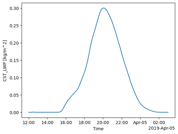
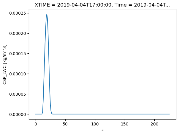
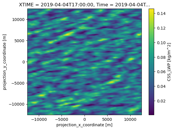
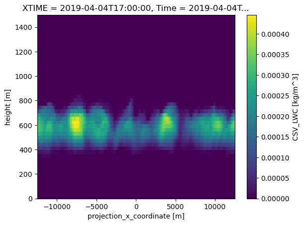
Plot wind speed
Let’s start with the first 10 files from the WRF simulation.
# Note the extra details required by open_mfdataset to connect the files together in time.
ds_wrf = xr.open_mfdataset(wrfout_file_list[:10],
                           combine="nested",
                           concat_dim="Time")
Since we did not use xwrf, this time, let’s fix the times.
ds_wrf["Time"] = ds_wrf["XTIME"]
/Users/mgrover/mambaforge/envs/lasso-those-clouds-cookbook-dev/lib/python3.12/site-packages/distributed/client.py:3164: UserWarning: Sending large graph of size 50.03 MiB.
This may cause some slowdown.
Consider scattering data ahead of time and using futures.
  warnings.warn(
2024-06-14 11:17:32,730 - distributed.nanny - ERROR - Worker process died unexpectedly
Visualize the Wind Vectors and Expose Destaggering
Next, we plot wind vectors at a selected level to demonstrate how to destagger the wind components to cell-center values with xarray. The destaggering is something that we can automatically handle with xwrf, but we explain the process below to be more transparent, especially with winds that are not in the cell-centers.
Destagger and Rename Dimensions
We need to:
destagger to cell centers
rename the staggered dimension back to the non-staggered name to avoid dimension conflicts
(re)name the unstaggered wind for convenience
Then, we are able to put these new DataArrays back into the ds_wrf Dataset.
# Plot wind vectors at a selected level to demonstrate how to destagger the wind components to cell-center values with xarray...

plot_level = 12  # index of level to plot
skip_xy = 10  # Sampling interval for the vector thinning

nt, nz, ny, nx = ds_wrf["T"].shape

ds_wrf["UA"] = 0.5*( ds_wrf["U"].isel(west_east_stag=slice(0, nx)) +
                    ds_wrf["U"].shift(west_east_stag=-1).isel(west_east_stag=slice(0, nx)) ).\
                    rename("UA").rename(west_east_stag="west_east")
ds_wrf["VA"] = 0.5*( ds_wrf["V"].isel(south_north_stag=slice(0, ny)) +
                    ds_wrf["V"].shift(south_north_stag=-1).isel(south_north_stag=slice(0, ny)) ).\
                    rename("VA").rename(south_north_stag="south_north")
ds_wrf["SPD"] = np.sqrt(ds_wrf["UA"]**2 + ds_wrf["VA"]**2).rename("wind speed").\
                    assign_attrs(units="m s-1", description="wind speed")
Visualize the Speed and Wind Vectors
Now, we can proceed to more plotting-specific data manipulation. We need to add spatial variables for the idealized domain (since XLAT and XLONG are constant in the file). This is needed by the xarray quiver routine.
Then, thin the grid to reduce the number of arrrows.
ds_wrf["west_east"] = xr.DataArray(data=np.arange(nx)*ds_wrf.attrs["DX"], dims="west_east", name="west_east", attrs={"units": "m"})
ds_wrf["south_north"] = xr.DataArray(data=np.arange(ny)*ds_wrf.attrs["DX"], dims="south_north", name="south_north", attrs={"units": "m"})

ds_wrf_thinned = ds_wrf.\
    isel(west_east=slice(0, nx, skip_xy), south_north=slice(0, ny, skip_xy), bottom_top=plot_level).\
    sel(Time=f"{case_date:%Y-%m-%d} {hour_to_plot}:00")

fig, ax = plt.subplots(ncols=1)
ds_wrf_thinned["SPD"].plot(ax=ax, x="west_east", y="south_north")
ds_wrf_thinned.plot.quiver(ax=ax, x="west_east", y="south_north", u="UA", v="VA",
                           scale=100)
plt.show()
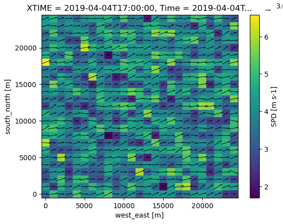
Compare with Observational Data from ARM
Now that we have plotted the simulation data from WRF, let’s take a look at the observations.
fs.glob(f"{path}/*")
['pythia/lasso-sgp/high_res_obs',
 'pythia/lasso-sgp/metrics',
 'pythia/lasso-sgp/sim0001',
 'pythia/lasso-sgp/sim0002',
 'pythia/lasso-sgp/sim0003',
 'pythia/lasso-sgp/sim0004',
 'pythia/lasso-sgp/sim0005',
 'pythia/lasso-sgp/sim0006',
 'pythia/lasso-sgp/sim0007',
 'pythia/lasso-sgp/sim0008']
fs.glob('pythia/lasso-sgp/high_res_obs/sgp*')
['pythia/lasso-sgp/high_res_obs/sgp915rwpwindcon10mC1.c1',
 'pythia/lasso-sgp/high_res_obs/sgp915rwpwindcon10mI10.c1',
 'pythia/lasso-sgp/high_res_obs/sgp915rwpwindcon10mI8.c1',
 'pythia/lasso-sgp/high_res_obs/sgp915rwpwindcon10mI9.c1',
 'pythia/lasso-sgp/high_res_obs/sgpcldfraccogs01mC1.c1',
 'pythia/lasso-sgp/high_res_obs/sgpcldfraccogs10mC1.c1',
 'pythia/lasso-sgp/high_res_obs/sgpcldfracset01mC1.c1',
 'pythia/lasso-sgp/high_res_obs/sgpcldfracset05mC1.c1',
 'pythia/lasso-sgp/high_res_obs/sgpcldfracset15mC1.c1',
 'pythia/lasso-sgp/high_res_obs/sgplassoblthermoC1.c1',
 'pythia/lasso-sgp/high_res_obs/sgplassodlcbhshcuC1.c1',
 'pythia/lasso-sgp/high_res_obs/sgplassodlcbhshcuE32.c1',
 'pythia/lasso-sgp/high_res_obs/sgplassodlcbhshcuE37.c1',
 'pythia/lasso-sgp/high_res_obs/sgplassodlcbhshcuE39.c1',
 'pythia/lasso-sgp/high_res_obs/sgplassodlcbhshcuE41.c1',
 'pythia/lasso-sgp/high_res_obs/sgplassolwpC1.c1',
 'pythia/lasso-sgp/high_res_obs/sgplclC1.c1']
# Compare with ARM Observational Data

import os

from arm_test_data import DATASETS
import matplotlib.pyplot as plt

import act

# Place your username and token here
username = os.getenv('ARM_USERNAME')
token = os.getenv('ARM_PASSWORD')

# If the username and token are not set, use the existing sample file
if username is None or token is None or len(username) == 0 or len(token) == 0:
    filename_ceil = DATASETS.fetch('sgpceilC1.b1.20190101.000000.nc')
    ceil_ds = act.io.arm.read_arm_netcdf(filename_ceil, engine='netcdf4')
else:
    # Example to show how easy it is to download ARM data if a username/token are set
    results = act.discovery.download_arm_data(
        username, token, 'sgpceilC1.b1', '2022-01-14', '2022-01-19'
    )
    ceil_ds = act.io.arm.read_arm_netcdf(results)

# Adjust ceilometer data for plotting
ceil_ds = act.corrections.ceil.correct_ceil(ceil_ds, -9999.0)

# Plot up ceilometer backscatter using HomeyerRainbow CVD friendly colormap
# The same could be done with keyword 'cmap='HomeyerRainbow'
display = act.plotting.TimeSeriesDisplay(ceil_ds, subplot_shape=(1,), figsize=(15, 5))
display.plot('backscatter', subplot_index=(0,), cvd_friendly=True)
plt.show()
/opt/conda/lib/python3.11/site-packages/dask/core.py:127: RuntimeWarning: invalid value encountered in log10
  return func(*(_execute_task(a, cache) for a in args))
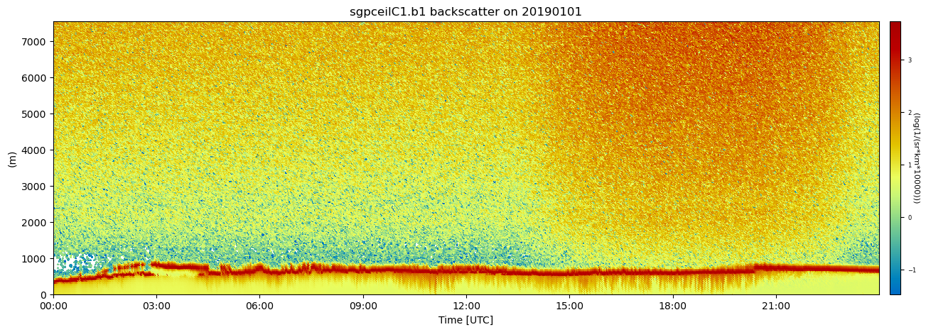
# ARM Plotting v2
import act
import numpy as np
import xarray as xr
import matplotlib.pyplot as plt
Plot Desired Variables
# Set your username and token here!
username = '***'
token = '***'

# Set the datastream and start/enddates
datastream = 'sgpaosmetE13.a1'
startdate = '2019-04-04'
enddate = '2019-04-05'

# Use ACT to easily download the data.  Watch for the data citation!  Show some support
# for ARM's instrument experts and cite their data if you use it in a publication
result = act.discovery.download_arm_data(username, token, datastream, startdate, enddate)
[DOWNLOADING] sgpaosmetE13.a1.20190404.000000.nc

If you use these data to prepare a publication, please cite:

Kyrouac, J., Springston, S., & Tuftedal, M. Meteorological Measurements
associated with the Aerosol Observing System (AOSMET). Atmospheric Radiation
Measurement (ARM) User Facility. https://doi.org/10.5439/1984920
# Let's read in the data using ACT and check out the data
ds_mpl = act.io.read_arm_netcdf(result)

ds_mpl
<xarray.Dataset> Size: 6MB
Dimensions:              (time: 86399)
Coordinates:
  * time                 (time) datetime64[ns] 691kB 2019-04-04T00:00:00.2200...
Data variables: (12/17)
    base_time            datetime64[ns] 8B 2019-04-04
    time_offset          (time) datetime64[ns] 691kB 2019-04-04T00:00:00.2200...
    rh_ambient           (time) float32 346kB dask.array<chunksize=(86399,), meta=np.ndarray>
    temperature_ambient  (time) float32 346kB dask.array<chunksize=(86399,), meta=np.ndarray>
    pressure_ambient     (time) float32 346kB dask.array<chunksize=(86399,), meta=np.ndarray>
    wind_speed           (time) float32 346kB dask.array<chunksize=(86399,), meta=np.ndarray>
    ...                   ...
    heater_volts         (time) float32 346kB dask.array<chunksize=(86399,), meta=np.ndarray>
    supply_volts         (time) float32 346kB dask.array<chunksize=(86399,), meta=np.ndarray>
    ref_volts            (time) float32 346kB dask.array<chunksize=(86399,), meta=np.ndarray>
    lat                  float32 4B ...
    lon                  float32 4B ...
    alt                  float32 4B ...
Attributes: (12/23)
    command_line:                aosmet_ingest -s sgp -f E13
    Conventions:                 ARM-1.2
    process_version:             ingest-aosmet-1.0-0.el6
    dod_version:                 aosmet-a1-2.2
    input_source:                /data/collection/sgp/sgpaosmetE13.00/sgpaosE...
    site_id:                     sgp
    ...                          ...
    doi:                         10.5439/1325987
    history:                     created by user dsmgr on machine ruby at 201...
    _file_dates:                 ['20190404']
    _file_times:                 ['000000']
    _datastream:                 sgpaosmetE13.a1
_arm_standards_flag: 1- time: 86399
- time(time)datetime64[ns]2019-04-04T00:00:00.220000 ... 2...
- long_name :
- Time offset from midnight
- standard_name :
- time
array(['2019-04-04T00:00:00.220000000', '2019-04-04T00:00:01.220000000',
       '2019-04-04T00:00:02.220000000', ..., '2019-04-04T23:59:57.160000000',
       '2019-04-04T23:59:58.160000000', '2019-04-04T23:59:59.160000000'],
      dtype='datetime64[ns]')
- base_time()datetime64[ns]2019-04-04
- string :
- 2019-04-04 00:00:00 0:00
- long_name :
- Base time in Epoch
- ancillary_variables :
- time_offset
array('2019-04-04T00:00:00.000000000', dtype='datetime64[ns]') - time_offset(time)datetime64[ns]2019-04-04T00:00:00.220000 ... 2...
- long_name :
- Time offset from base_time
- ancillary_variables :
- base_time
array(['2019-04-04T00:00:00.220000000', '2019-04-04T00:00:01.220000000', '2019-04-04T00:00:02.220000000', ..., '2019-04-04T23:59:57.160000000', '2019-04-04T23:59:58.160000000', '2019-04-04T23:59:59.160000000'], dtype='datetime64[ns]') - rh_ambient(time)float32dask.array<chunksize=(86399,), meta=np.ndarray>
- long_name :
- Ambient air relative humidity
- units :
- %
- standard_name :
- relative_humidity
Array Chunk Bytes 337.50 kiB 337.50 kiB Shape (86399,) (86399,) Dask graph 1 chunks in 2 graph layers Data type float32 numpy.ndarray - temperature_ambient(time)float32dask.array<chunksize=(86399,), meta=np.ndarray>
- long_name :
- Ambient air temperature
- units :
- degC
- standard_name :
- air_temperature
Array Chunk Bytes 337.50 kiB 337.50 kiB Shape (86399,) (86399,) Dask graph 1 chunks in 2 graph layers Data type float32 numpy.ndarray - pressure_ambient(time)float32dask.array<chunksize=(86399,), meta=np.ndarray>
- long_name :
- Ambient pressure
- units :
- hPa
- standard_name :
- surface_air_pressure
Array Chunk Bytes 337.50 kiB 337.50 kiB Shape (86399,) (86399,) Dask graph 1 chunks in 2 graph layers Data type float32 numpy.ndarray - wind_speed(time)float32dask.array<chunksize=(86399,), meta=np.ndarray>
- long_name :
- Wind speed
- units :
- m/s
- standard_name :
- wind_speed
Array Chunk Bytes 337.50 kiB 337.50 kiB Shape (86399,) (86399,) Dask graph 1 chunks in 2 graph layers Data type float32 numpy.ndarray - wind_direction(time)float32dask.array<chunksize=(86399,), meta=np.ndarray>
- long_name :
- Wind direction, relative to true North
- units :
- degree
- standard_name :
- wind_from_direction
Array Chunk Bytes 337.50 kiB 337.50 kiB Shape (86399,) (86399,) Dask graph 1 chunks in 2 graph layers Data type float32 numpy.ndarray - rain_amount(time)float32dask.array<chunksize=(86399,), meta=np.ndarray>
- long_name :
- Rain amount
- units :
- mm/s
- standard_name :
- rainfall_rate
Array Chunk Bytes 337.50 kiB 337.50 kiB Shape (86399,) (86399,) Dask graph 1 chunks in 2 graph layers Data type float32 numpy.ndarray - rain_duration(time)float32dask.array<chunksize=(86399,), meta=np.ndarray>
- long_name :
- Rain duration
- units :
- s
Array Chunk Bytes 337.50 kiB 337.50 kiB Shape (86399,) (86399,) Dask graph 1 chunks in 2 graph layers Data type float32 numpy.ndarray - rain_intensity(time)float32dask.array<chunksize=(86399,), meta=np.ndarray>
- long_name :
- Rain intensity
- units :
- mm/hr
Array Chunk Bytes 337.50 kiB 337.50 kiB Shape (86399,) (86399,) Dask graph 1 chunks in 2 graph layers Data type float32 numpy.ndarray - heater_temp(time)float32dask.array<chunksize=(86399,), meta=np.ndarray>
- long_name :
- Heater temperature
- units :
- degC
Array Chunk Bytes 337.50 kiB 337.50 kiB Shape (86399,) (86399,) Dask graph 1 chunks in 2 graph layers Data type float32 numpy.ndarray - heater_volts(time)float32dask.array<chunksize=(86399,), meta=np.ndarray>
- long_name :
- Heater voltage
- units :
- V
Array Chunk Bytes 337.50 kiB 337.50 kiB Shape (86399,) (86399,) Dask graph 1 chunks in 2 graph layers Data type float32 numpy.ndarray - supply_volts(time)float32dask.array<chunksize=(86399,), meta=np.ndarray>
- long_name :
- Supply voltage
- units :
- V
Array Chunk Bytes 337.50 kiB 337.50 kiB Shape (86399,) (86399,) Dask graph 1 chunks in 2 graph layers Data type float32 numpy.ndarray - ref_volts(time)float32dask.array<chunksize=(86399,), meta=np.ndarray>
- long_name :
- Reference voltage
- units :
- V
Array Chunk Bytes 337.50 kiB 337.50 kiB Shape (86399,) (86399,) Dask graph 1 chunks in 2 graph layers Data type float32 numpy.ndarray - lat()float32...
- long_name :
- North latitude
- units :
- degree_N
- valid_min :
- -90.0
- valid_max :
- 90.0
- standard_name :
- latitude
[1 values with dtype=float32]
- lon()float32...
- long_name :
- East longitude
- units :
- degree_E
- valid_min :
- -180.0
- valid_max :
- 180.0
- standard_name :
- longitude
[1 values with dtype=float32]
- alt()float32...
- long_name :
- Altitude above mean sea level
- units :
- m
- standard_name :
- altitude
[1 values with dtype=float32]
- timePandasIndex
PandasIndex(DatetimeIndex(['2019-04-04 00:00:00.220000', '2019-04-04 00:00:01.220000',
               '2019-04-04 00:00:02.220000', '2019-04-04 00:00:03.220000',
               '2019-04-04 00:00:04.220000', '2019-04-04 00:00:05.220000',
               '2019-04-04 00:00:06.220000', '2019-04-04 00:00:07.220000',
               '2019-04-04 00:00:08.220000', '2019-04-04 00:00:09.220000',
               ...
               '2019-04-04 23:59:50.160000', '2019-04-04 23:59:51.160000',
               '2019-04-04 23:59:52.160000', '2019-04-04 23:59:53.160000',
               '2019-04-04 23:59:54.160000', '2019-04-04 23:59:55.160000',
               '2019-04-04 23:59:56.160000', '2019-04-04 23:59:57.160000',
               '2019-04-04 23:59:58.160000', '2019-04-04 23:59:59.160000'],
              dtype='datetime64[ns]', name='time', length=86399, freq=None))
- command_line :
- aosmet_ingest -s sgp -f E13
- Conventions :
- ARM-1.2
- process_version :
- ingest-aosmet-1.0-0.el6
- dod_version :
- aosmet-a1-2.2
- input_source :
- /data/collection/sgp/sgpaosmetE13.00/sgpaosE13.met.01s.00.20190404.000000.raw.tsv
- site_id :
- sgp
- platform_id :
- aosmet
- facility_id :
- E13
- data_level :
- a1
- location_description :
- Southern Great Plains (SGP), Lamont, Oklahoma
- datastream :
- sgpaosmetE13.a1
- serial_number :
- K/WD
- sampling_interval :
- 1 second
- met_instrument_description :
- WXT520
- instrument_manufacturer :
- N/A
- mentor_name :
- Kyrouac
- mentor_affiliation :
- ANL
- doi :
- 10.5439/1325987
- history :
- created by user dsmgr on machine ruby at 2019-04-04 01:22:00, using ingest-aosmet-1.0-0.el6
- _file_dates :
- ['20190404']
- _file_times :
- ['000000']
- _datastream :
- sgpaosmetE13.a1
- _arm_standards_flag :
- 1
Change variable (as desired), Apply QC, and Plot Again
# Let's take a look at the quality control information associated with a variable from the MPL
variable = 'temperature_ambient'

# First, for many of the ACT QC features, we need to get the dataset more to CF standard and that
# involves cleaning up some of the attributes and ways that ARM has historically handled QC
ds_mpl.clean.cleanup()

# Apply corrections for the ceilometer, correcting for the vertical height
#ds_mpl = act.corrections.ceil.correct_ceil(ds_mpl,-999.0)

# Next, let's take a look at visualizing the quality control information
# Create a plotting display object with 2 plots
display = act.plotting.TimeSeriesDisplay(ds_mpl, figsize=(10, 5), subplot_shape=(1,))

# # Plot up the variable in the first plot
display.plot(variable, subplot_index=(0,))

# # Plot up the QC variable in the second plot
# #display.qc_flag_block_plot(variable, subplot_index=(1,))
# plt.show()
<Axes: title={'center': 'sgpaosmetE13.a1 temperature_ambient on 20190404'}, xlabel='Time [UTC]', ylabel='(degC)'>