Load in necessary packages
# Libraries required for moisture convergence visualization
from datetime import datetime
import numpy as np
import xarray as xr
import xwrf
import glob
import metpy.calc as mpcalc
import math

import matplotlib.pyplot as plt
We will first identify LASSO SGP case(s) of interest
# Define path to the lasso simulation data
path_shcu_root = "/data/project/ARM_Summer_School_2024_Data/lasso_tutorial/ShCu/untar"  # on Jupyter

#Define LASSO SGP case date and simulation of interest
case_date = datetime(2019, 4, 4) #Options[April 4, 2019; May 6, 2019]
sim_id = 4

#Load in LASSO wrfstat files. These provide 10-minute averages for various metorology variables and diagnostics
ds_stat = xr.open_dataset(f"{path_shcu_root}/{case_date:%Y%m%d}/sim{sim_id:04d}/raw_model/wrfstat_d01_{case_date:%Y-%m-%d_12:00:00}.nc")
#ds_stat

#Load in LASSO-ShCu wrfout data, which is raw simulation output from the Weather Research and Forecasting (WRF) model run in an idealized LES mode.
#Post process using xwrf package
ds = xr.open_mfdataset(f"{path_shcu_root}/{case_date:%Y%m%d}/sim{sim_id:04d}/raw_model/wrfout_d01_*.nc", combine="nested", concat_dim="Time").xwrf.postprocess()

# By default, xarray does not interpret the wrfout/wrfstat time information in a way that attaches
# it to each variable. Here is a trick to map the time held in XTIME with the Time coordinate
# associated with each variable.
ds_stat["Time"] = ds_stat["XTIME"]
ds["Time"] = ds["XTIME"]
ds
<xarray.Dataset> Size: 255GB
Dimensions:                    (Time: 91, y: 250, x: 250, soil_layers_stag: 5,
                                z: 226, x_stag: 251, y_stag: 251, z_stag: 227,
                                force_layers: 751)
Coordinates: (12/15)
    CLAT                       (y, x) float32 250kB dask.array<chunksize=(125, 125), meta=np.ndarray>
    XLAT                       (y, x) float32 250kB dask.array<chunksize=(125, 125), meta=np.ndarray>
    XLONG                      (y, x) float32 250kB dask.array<chunksize=(125, 125), meta=np.ndarray>
    XTIME                      (Time) datetime64[ns] 728B dask.array<chunksize=(6,), meta=np.ndarray>
    XLAT_U                     (y, x_stag) float32 251kB dask.array<chunksize=(125, 126), meta=np.ndarray>
    XLONG_U                    (y, x_stag) float32 251kB dask.array<chunksize=(125, 126), meta=np.ndarray>
    ...                         ...
  * z_stag                     (z_stag) float32 908B 1.0 0.9959 ... 0.002178 0.0
  * Time                       (Time) datetime64[ns] 728B 2019-04-04T12:00:00...
  * y_stag                     (y_stag) float64 2kB -1.25e+04 ... 1.25e+04
  * y                          (y) float64 2kB -1.245e+04 ... 1.245e+04
  * x                          (x) float64 2kB -1.245e+04 ... 1.245e+04
  * x_stag                     (x_stag) float64 2kB -1.25e+04 ... 1.25e+04
Dimensions without coordinates: soil_layers_stag, force_layers
Data variables: (12/251)
    Times                      (Time) |S19 2kB dask.array<chunksize=(1,), meta=np.ndarray>
    LU_INDEX                   (Time, y, x) float32 23MB dask.array<chunksize=(1, 125, 125), meta=np.ndarray>
    ZS                         (Time, soil_layers_stag) float32 2kB dask.array<chunksize=(1, 5), meta=np.ndarray>
    DZS                        (Time, soil_layers_stag) float32 2kB dask.array<chunksize=(1, 5), meta=np.ndarray>
    VAR_SSO                    (Time, y, x) float32 23MB dask.array<chunksize=(1, 125, 125), meta=np.ndarray>
    U                          (Time, z, y, x_stag) float32 5GB dask.array<chunksize=(1, 226, 125, 126), meta=np.ndarray>
    ...                         ...
    geopotential               (Time, z_stag, y, x) float32 5GB dask.array<chunksize=(1, 227, 125, 125), meta=np.ndarray>
    geopotential_height        (Time, z_stag, y, x) float32 5GB dask.array<chunksize=(1, 227, 125, 125), meta=np.ndarray>
    wind_east                  (Time, z, y, x) float32 5GB dask.array<chunksize=(1, 226, 125, 125), meta=np.ndarray>
    wind_north                 (Time, z, y, x) float32 5GB dask.array<chunksize=(1, 226, 125, 125), meta=np.ndarray>
    wind_east_10               (Time, y, x) float32 23MB dask.array<chunksize=(1, 125, 125), meta=np.ndarray>
    wind_north_10              (Time, y, x) float32 23MB dask.array<chunksize=(1, 125, 125), meta=np.ndarray>
Attributes: (12/142)
    TITLE:                                  OUTPUT FROM WRF V3.8.1 MODEL
    START_DATE:                            2019-04-04_12:00:00
    SIMULATION_START_DATE:                 2019-04-04_12:00:00
    WEST-EAST_GRID_DIMENSION:              251
    SOUTH-NORTH_GRID_DIMENSION:            251
    BOTTOM-TOP_GRID_DIMENSION:             227
    ...                                    ...
    config_aerosol:                        NA
    config_forecast_time:                  15.0 h
    config_boundary_method:                Periodic
    config_microphysics:                   Thompson (mp_physics=8)
    config_nickname:                       runlas20190404v1addhm
    simulation_origin_host:                cumulus-login2.ccs.ornl.gov
xarray.Dataset
- Time: 91
- y: 250
- x: 250
- soil_layers_stag: 5
- z: 226
- x_stag: 251
- y_stag: 251
- z_stag: 227
- force_layers: 751
- CLAT(y, x)float32dask.array<chunksize=(125, 125), meta=np.ndarray>
- FieldType :
- 104
- MemoryOrder :
- XY
- description :
- COMPUTATIONAL GRID LATITUDE, SOUTH IS NEGATIVE
- units :
- degree_north
- stagger :
Array Chunk Bytes 244.14 kiB 61.04 kiB Shape (250, 250) (125, 125) Dask graph 4 chunks in 34 graph layers Data type float32 numpy.ndarray - XLAT(y, x)float32dask.array<chunksize=(125, 125), meta=np.ndarray>
- FieldType :
- 104
- MemoryOrder :
- XY
- description :
- LATITUDE, SOUTH IS NEGATIVE
- units :
- degree_north
- stagger :
Array Chunk Bytes 244.14 kiB 61.04 kiB Shape (250, 250) (125, 125) Dask graph 4 chunks in 34 graph layers Data type float32 numpy.ndarray - XLONG(y, x)float32dask.array<chunksize=(125, 125), meta=np.ndarray>
- FieldType :
- 104
- MemoryOrder :
- XY
- description :
- LONGITUDE, WEST IS NEGATIVE
- units :
- degree_east
- stagger :
Array Chunk Bytes 244.14 kiB 61.04 kiB Shape (250, 250) (125, 125) Dask graph 4 chunks in 34 graph layers Data type float32 numpy.ndarray - XTIME(Time)datetime64[ns]dask.array<chunksize=(6,), meta=np.ndarray>
- FieldType :
- 104
- MemoryOrder :
- 0
- description :
- minutes since 2019-04-04 12:00:00
- stagger :
Array Chunk Bytes 728 B 48 B Shape (91,) (6,) Dask graph 16 chunks in 33 graph layers Data type datetime64[ns] numpy.ndarray - XLAT_U(y, x_stag)float32dask.array<chunksize=(125, 126), meta=np.ndarray>
- FieldType :
- 104
- MemoryOrder :
- XY
- description :
- LATITUDE, SOUTH IS NEGATIVE
- units :
- degree_north
- stagger :
- X
Array Chunk Bytes 245.12 kiB 61.52 kiB Shape (250, 251) (125, 126) Dask graph 4 chunks in 34 graph layers Data type float32 numpy.ndarray - XLONG_U(y, x_stag)float32dask.array<chunksize=(125, 126), meta=np.ndarray>
- FieldType :
- 104
- MemoryOrder :
- XY
- description :
- LONGITUDE, WEST IS NEGATIVE
- units :
- degree_east
- stagger :
- X
Array Chunk Bytes 245.12 kiB 61.52 kiB Shape (250, 251) (125, 126) Dask graph 4 chunks in 34 graph layers Data type float32 numpy.ndarray - XLAT_V(y_stag, x)float32dask.array<chunksize=(126, 125), meta=np.ndarray>
- FieldType :
- 104
- MemoryOrder :
- XY
- description :
- LATITUDE, SOUTH IS NEGATIVE
- units :
- degree_north
- stagger :
- Y
Array Chunk Bytes 245.12 kiB 61.52 kiB Shape (251, 250) (126, 125) Dask graph 4 chunks in 34 graph layers Data type float32 numpy.ndarray - XLONG_V(y_stag, x)float32dask.array<chunksize=(126, 125), meta=np.ndarray>
- FieldType :
- 104
- MemoryOrder :
- XY
- description :
- LONGITUDE, WEST IS NEGATIVE
- units :
- degree_east
- stagger :
- Y
Array Chunk Bytes 245.12 kiB 61.52 kiB Shape (251, 250) (126, 125) Dask graph 4 chunks in 34 graph layers Data type float32 numpy.ndarray - z(z)float320.9979 0.9938 ... 0.005743 0.001089
- FieldType :
- 104
- MemoryOrder :
- Z
- description :
- eta values on half (mass) levels
- units :
- stagger :
- axis :
- Z
- standard_name :
- atmosphere_sigma_coordinate
array([0.997944, 0.993847, 0.989777, ..., 0.01304 , 0.005743, 0.001089], dtype=float32) - z_stag(z_stag)float321.0 0.9959 0.9918 ... 0.002178 0.0
- FieldType :
- 104
- MemoryOrder :
- Z
- description :
- eta values on full (w) levels
- units :
- stagger :
- Z
- axis :
- Z
- c_grid_axis_shift :
- 0.5
- standard_name :
- atmosphere_sigma_coordinate
array([1. , 0.995887, 0.991808, ..., 0.009308, 0.002178, 0. ], dtype=float32) - Time(Time)datetime64[ns]2019-04-04T12:00:00 ... 2019-04-...
- FieldType :
- 104
- MemoryOrder :
- 0
- description :
- minutes since 2019-04-04 12:00:00
- stagger :
array(['2019-04-04T12:00:00.000000000', '2019-04-04T12:10:00.000000000', '2019-04-04T12:20:00.000000000', '2019-04-04T12:30:00.000000000', '2019-04-04T12:40:00.000000000', '2019-04-04T12:50:00.000000000', '2019-04-04T13:00:00.000000000', '2019-04-04T13:10:00.000000000', '2019-04-04T13:20:00.000000000', '2019-04-04T13:30:00.000000000', '2019-04-04T13:40:00.000000000', '2019-04-04T13:50:00.000000000', '2019-04-04T14:00:00.000000000', '2019-04-04T14:10:00.000000000', '2019-04-04T14:20:00.000000000', '2019-04-04T14:30:00.000000000', '2019-04-04T14:40:00.000000000', '2019-04-04T14:50:00.000000000', '2019-04-04T15:00:00.000000000', '2019-04-04T15:10:00.000000000', '2019-04-04T15:20:00.000000000', '2019-04-04T15:30:00.000000000', '2019-04-04T15:40:00.000000000', '2019-04-04T15:50:00.000000000', '2019-04-04T16:00:00.000000000', '2019-04-04T16:10:00.000000000', '2019-04-04T16:20:00.000000000', '2019-04-04T16:30:00.000000000', '2019-04-04T16:40:00.000000000', '2019-04-04T16:50:00.000000000', '2019-04-04T17:00:00.000000000', '2019-04-04T17:10:00.000000000', '2019-04-04T17:20:00.000000000', '2019-04-04T17:30:00.000000000', '2019-04-04T17:40:00.000000000', '2019-04-04T17:50:00.000000000', '2019-04-04T18:00:00.000000000', '2019-04-04T18:10:00.000000000', '2019-04-04T18:20:00.000000000', '2019-04-04T18:30:00.000000000', '2019-04-04T18:40:00.000000000', '2019-04-04T18:50:00.000000000', '2019-04-04T19:00:00.000000000', '2019-04-04T19:10:00.000000000', '2019-04-04T19:20:00.000000000', '2019-04-04T19:30:00.000000000', '2019-04-04T19:40:00.000000000', '2019-04-04T19:50:00.000000000', '2019-04-04T20:00:00.000000000', '2019-04-04T20:10:00.000000000', '2019-04-04T20:20:00.000000000', '2019-04-04T20:30:00.000000000', '2019-04-04T20:40:00.000000000', '2019-04-04T20:50:00.000000000', '2019-04-04T21:00:00.000000000', '2019-04-04T21:10:00.000000000', '2019-04-04T21:20:00.000000000', '2019-04-04T21:30:00.000000000', '2019-04-04T21:40:00.000000000', '2019-04-04T21:50:00.000000000', '2019-04-04T22:00:00.000000000', '2019-04-04T22:10:00.000000000', '2019-04-04T22:20:00.000000000', '2019-04-04T22:30:00.000000000', '2019-04-04T22:40:00.000000000', '2019-04-04T22:50:00.000000000', '2019-04-04T23:00:00.000000000', '2019-04-04T23:10:00.000000000', '2019-04-04T23:20:00.000000000', '2019-04-04T23:30:00.000000000', '2019-04-04T23:40:00.000000000', '2019-04-04T23:50:00.000000000', '2019-04-05T00:00:00.000000000', '2019-04-05T00:10:00.000000000', '2019-04-05T00:20:00.000000000', '2019-04-05T00:30:00.000000000', '2019-04-05T00:40:00.000000000', '2019-04-05T00:50:00.000000000', '2019-04-05T01:00:00.000000000', '2019-04-05T01:10:00.000000000', '2019-04-05T01:20:00.000000000', '2019-04-05T01:30:00.000000000', '2019-04-05T01:40:00.000000000', '2019-04-05T01:50:00.000000000', '2019-04-05T02:00:00.000000000', '2019-04-05T02:10:00.000000000', '2019-04-05T02:20:00.000000000', '2019-04-05T02:30:00.000000000', '2019-04-05T02:40:00.000000000', '2019-04-05T02:50:00.000000000', '2019-04-05T03:00:00.000000000'], dtype='datetime64[ns]') - y_stag(y_stag)float64-1.25e+04 -1.24e+04 ... 1.25e+04
- units :
- m
- standard_name :
- projection_y_coordinate
- axis :
- Y
- c_grid_axis_shift :
- 0.5
array([-12500., -12400., -12300., ..., 12300., 12400., 12500.])
- y(y)float64-1.245e+04 -1.235e+04 ... 1.245e+04
- units :
- m
- standard_name :
- projection_y_coordinate
- axis :
- Y
array([-12450., -12350., -12250., ..., 12250., 12350., 12450.])
- x(x)float64-1.245e+04 -1.235e+04 ... 1.245e+04
- units :
- m
- standard_name :
- projection_x_coordinate
- axis :
- X
array([-12450., -12350., -12250., ..., 12250., 12350., 12450.])
- x_stag(x_stag)float64-1.25e+04 -1.24e+04 ... 1.25e+04
- units :
- m
- standard_name :
- projection_x_coordinate
- axis :
- X
- c_grid_axis_shift :
- 0.5
array([-12500., -12400., -12300., ..., 12300., 12400., 12500.])
- Times(Time)|S19dask.array<chunksize=(1,), meta=np.ndarray>
Array Chunk Bytes 1.69 kiB 19 B Shape (91,) (1,) Dask graph 91 chunks in 33 graph layers Data type |S19 numpy.ndarray - LU_INDEX(Time, y, x)float32dask.array<chunksize=(1, 125, 125), meta=np.ndarray>
- FieldType :
- 104
- MemoryOrder :
- XY
- description :
- LAND USE CATEGORY
- units :
- stagger :
Array Chunk Bytes 21.70 MiB 61.04 kiB Shape (91, 250, 250) (1, 125, 125) Dask graph 364 chunks in 33 graph layers Data type float32 numpy.ndarray - ZS(Time, soil_layers_stag)float32dask.array<chunksize=(1, 5), meta=np.ndarray>
- FieldType :
- 104
- MemoryOrder :
- Z
- description :
- DEPTHS OF CENTERS OF SOIL LAYERS
- units :
- m
- stagger :
- Z
Array Chunk Bytes 1.78 kiB 20 B Shape (91, 5) (1, 5) Dask graph 91 chunks in 33 graph layers Data type float32 numpy.ndarray - DZS(Time, soil_layers_stag)float32dask.array<chunksize=(1, 5), meta=np.ndarray>
- FieldType :
- 104
- MemoryOrder :
- Z
- description :
- THICKNESSES OF SOIL LAYERS
- units :
- m
- stagger :
- Z
Array Chunk Bytes 1.78 kiB 20 B Shape (91, 5) (1, 5) Dask graph 91 chunks in 33 graph layers Data type float32 numpy.ndarray - VAR_SSO(Time, y, x)float32dask.array<chunksize=(1, 125, 125), meta=np.ndarray>
- FieldType :
- 104
- MemoryOrder :
- XY
- description :
- Variance of Subgrid Scale Orography MSL
- units :
- m2
- stagger :
Array Chunk Bytes 21.70 MiB 61.04 kiB Shape (91, 250, 250) (1, 125, 125) Dask graph 364 chunks in 33 graph layers Data type float32 numpy.ndarray - U(Time, z, y, x_stag)float32dask.array<chunksize=(1, 226, 125, 126), meta=np.ndarray>
- FieldType :
- 104
- MemoryOrder :
- XYZ
- description :
- x-wind component
- units :
- m s-1
- stagger :
- X
- standard_name :
- x_wind
Array Chunk Bytes 4.81 GiB 13.58 MiB Shape (91, 226, 250, 251) (1, 226, 125, 126) Dask graph 364 chunks in 33 graph layers Data type float32 numpy.ndarray - V(Time, z, y_stag, x)float32dask.array<chunksize=(1, 226, 126, 125), meta=np.ndarray>
- FieldType :
- 104
- MemoryOrder :
- XYZ
- description :
- y-wind component
- units :
- m s-1
- stagger :
- Y
- standard_name :
- y_wind
Array Chunk Bytes 4.81 GiB 13.58 MiB Shape (91, 226, 251, 250) (1, 226, 126, 125) Dask graph 364 chunks in 33 graph layers Data type float32 numpy.ndarray - W(Time, z_stag, y, x)float32dask.array<chunksize=(1, 227, 125, 125), meta=np.ndarray>
- FieldType :
- 104
- MemoryOrder :
- XYZ
- description :
- z-wind component
- units :
- m s-1
- stagger :
- Z
- standard_name :
- upward_air_velocity
Array Chunk Bytes 4.81 GiB 13.53 MiB Shape (91, 227, 250, 250) (1, 227, 125, 125) Dask graph 364 chunks in 33 graph layers Data type float32 numpy.ndarray - HFX_FORCE(Time)float32dask.array<chunksize=(6,), meta=np.ndarray>
- FieldType :
- 104
- MemoryOrder :
- 0
- description :
- SCM ideal surface sensible heat flux
- units :
- W m-2
- stagger :
Array Chunk Bytes 364 B 24 B Shape (91,) (6,) Dask graph 16 chunks in 33 graph layers Data type float32 numpy.ndarray - LH_FORCE(Time)float32dask.array<chunksize=(6,), meta=np.ndarray>
- FieldType :
- 104
- MemoryOrder :
- 0
- description :
- SCM ideal surface latent heat flux
- units :
- W m-2
- stagger :
Array Chunk Bytes 364 B 24 B Shape (91,) (6,) Dask graph 16 chunks in 33 graph layers Data type float32 numpy.ndarray - TSK_FORCE(Time)float32dask.array<chunksize=(6,), meta=np.ndarray>
- FieldType :
- 104
- MemoryOrder :
- 0
- description :
- SCM ideal surface skin temperature
- units :
- W m-2
- stagger :
Array Chunk Bytes 364 B 24 B Shape (91,) (6,) Dask graph 16 chunks in 33 graph layers Data type float32 numpy.ndarray - HFX_FORCE_TEND(Time)float32dask.array<chunksize=(6,), meta=np.ndarray>
- FieldType :
- 104
- MemoryOrder :
- 0
- description :
- SCM ideal surface sensible heat flux tendency
- units :
- W m-2 s-1
- stagger :
Array Chunk Bytes 364 B 24 B Shape (91,) (6,) Dask graph 16 chunks in 33 graph layers Data type float32 numpy.ndarray - LH_FORCE_TEND(Time)float32dask.array<chunksize=(6,), meta=np.ndarray>
- FieldType :
- 104
- MemoryOrder :
- 0
- description :
- SCM ideal surface latent heat flux tendency
- units :
- W m-2 s-1
- stagger :
Array Chunk Bytes 364 B 24 B Shape (91,) (6,) Dask graph 16 chunks in 33 graph layers Data type float32 numpy.ndarray - TSK_FORCE_TEND(Time)float32dask.array<chunksize=(6,), meta=np.ndarray>
- FieldType :
- 104
- MemoryOrder :
- 0
- description :
- SCM ideal surface skin temperature tendency
- units :
- W m-2 s-1
- stagger :
Array Chunk Bytes 364 B 24 B Shape (91,) (6,) Dask graph 16 chunks in 33 graph layers Data type float32 numpy.ndarray - MU(Time, y, x)float32dask.array<chunksize=(1, 125, 125), meta=np.ndarray>
- FieldType :
- 104
- MemoryOrder :
- XY
- description :
- perturbation dry air mass in column
- units :
- Pa
- stagger :
Array Chunk Bytes 21.70 MiB 61.04 kiB Shape (91, 250, 250) (1, 125, 125) Dask graph 364 chunks in 33 graph layers Data type float32 numpy.ndarray - MUB(Time, y, x)float32dask.array<chunksize=(1, 125, 125), meta=np.ndarray>
- FieldType :
- 104
- MemoryOrder :
- XY
- description :
- base state dry air mass in column
- units :
- Pa
- stagger :
Array Chunk Bytes 21.70 MiB 61.04 kiB Shape (91, 250, 250) (1, 125, 125) Dask graph 364 chunks in 33 graph layers Data type float32 numpy.ndarray - NEST_POS(Time, y, x)float32dask.array<chunksize=(1, 125, 125), meta=np.ndarray>
- FieldType :
- 104
- MemoryOrder :
- XY
- description :
- -
- stagger :
Array Chunk Bytes 21.70 MiB 61.04 kiB Shape (91, 250, 250) (1, 125, 125) Dask graph 364 chunks in 33 graph layers Data type float32 numpy.ndarray - TKE(Time, z, y, x)float32dask.array<chunksize=(1, 226, 125, 125), meta=np.ndarray>
- FieldType :
- 104
- MemoryOrder :
- XYZ
- description :
- TURBULENCE KINETIC ENERGY
- units :
- m2 s-2
- stagger :
Array Chunk Bytes 4.79 GiB 13.47 MiB Shape (91, 226, 250, 250) (1, 226, 125, 125) Dask graph 364 chunks in 33 graph layers Data type float32 numpy.ndarray - ALT(Time, z, y, x)float32dask.array<chunksize=(1, 226, 125, 125), meta=np.ndarray>
- FieldType :
- 104
- MemoryOrder :
- XYZ
- description :
- inverse density
- units :
- m3 kg-1
- stagger :
Array Chunk Bytes 4.79 GiB 13.47 MiB Shape (91, 226, 250, 250) (1, 226, 125, 125) Dask graph 364 chunks in 33 graph layers Data type float32 numpy.ndarray - FNM(Time, z)float32dask.array<chunksize=(1, 226), meta=np.ndarray>
- FieldType :
- 104
- MemoryOrder :
- Z
- description :
- upper weight for vertical stretching
- units :
- stagger :
Array Chunk Bytes 80.34 kiB 904 B Shape (91, 226) (1, 226) Dask graph 91 chunks in 33 graph layers Data type float32 numpy.ndarray - FNP(Time, z)float32dask.array<chunksize=(1, 226), meta=np.ndarray>
- FieldType :
- 104
- MemoryOrder :
- Z
- description :
- lower weight for vertical stretching
- units :
- stagger :
Array Chunk Bytes 80.34 kiB 904 B Shape (91, 226) (1, 226) Dask graph 91 chunks in 33 graph layers Data type float32 numpy.ndarray - RDNW(Time, z)float32dask.array<chunksize=(1, 226), meta=np.ndarray>
- FieldType :
- 104
- MemoryOrder :
- Z
- description :
- inverse d(eta) values between full (w) levels
- units :
- stagger :
Array Chunk Bytes 80.34 kiB 904 B Shape (91, 226) (1, 226) Dask graph 91 chunks in 33 graph layers Data type float32 numpy.ndarray - RDN(Time, z)float32dask.array<chunksize=(1, 226), meta=np.ndarray>
- FieldType :
- 104
- MemoryOrder :
- Z
- description :
- inverse d(eta) values between half (mass) levels
- units :
- stagger :
Array Chunk Bytes 80.34 kiB 904 B Shape (91, 226) (1, 226) Dask graph 91 chunks in 33 graph layers Data type float32 numpy.ndarray - DNW(Time, z)float32dask.array<chunksize=(1, 226), meta=np.ndarray>
- FieldType :
- 104
- MemoryOrder :
- Z
- description :
- d(eta) values between full (w) levels
- units :
- stagger :
Array Chunk Bytes 80.34 kiB 904 B Shape (91, 226) (1, 226) Dask graph 91 chunks in 33 graph layers Data type float32 numpy.ndarray - DN(Time, z)float32dask.array<chunksize=(1, 226), meta=np.ndarray>
- FieldType :
- 104
- MemoryOrder :
- Z
- description :
- d(eta) values between half (mass) levels
- units :
- stagger :
Array Chunk Bytes 80.34 kiB 904 B Shape (91, 226) (1, 226) Dask graph 91 chunks in 33 graph layers Data type float32 numpy.ndarray - CFN(Time)float32dask.array<chunksize=(6,), meta=np.ndarray>
- FieldType :
- 104
- MemoryOrder :
- 0
- description :
- extrapolation constant
- units :
- stagger :
Array Chunk Bytes 364 B 24 B Shape (91,) (6,) Dask graph 16 chunks in 33 graph layers Data type float32 numpy.ndarray - CFN1(Time)float32dask.array<chunksize=(6,), meta=np.ndarray>
- FieldType :
- 104
- MemoryOrder :
- 0
- description :
- extrapolation constant
- units :
- stagger :
Array Chunk Bytes 364 B 24 B Shape (91,) (6,) Dask graph 16 chunks in 33 graph layers Data type float32 numpy.ndarray - THIS_IS_AN_IDEAL_RUN(Time)int32dask.array<chunksize=(6,), meta=np.ndarray>
- FieldType :
- 106
- MemoryOrder :
- 0
- description :
- T/F flag: this is an ARW ideal simulation
- stagger :
Array Chunk Bytes 364 B 24 B Shape (91,) (6,) Dask graph 16 chunks in 33 graph layers Data type int32 numpy.ndarray - P_HYD(Time, z, y, x)float32dask.array<chunksize=(1, 226, 125, 125), meta=np.ndarray>
- FieldType :
- 104
- MemoryOrder :
- XYZ
- description :
- hydrostatic pressure
- units :
- Pa
- stagger :
Array Chunk Bytes 4.79 GiB 13.47 MiB Shape (91, 226, 250, 250) (1, 226, 125, 125) Dask graph 364 chunks in 33 graph layers Data type float32 numpy.ndarray - Q2(Time, y, x)float32dask.array<chunksize=(1, 125, 125), meta=np.ndarray>
- FieldType :
- 104
- MemoryOrder :
- XY
- description :
- QV at 2 M
- units :
- kg kg-1
- stagger :
- standard_name :
- humidity_mixing_ratio
- long_name :
- humidity_mixing_ratio_at_2m_agl
Array Chunk Bytes 21.70 MiB 61.04 kiB Shape (91, 250, 250) (1, 125, 125) Dask graph 364 chunks in 33 graph layers Data type float32 numpy.ndarray - T2(Time, y, x)float32dask.array<chunksize=(1, 125, 125), meta=np.ndarray>
- FieldType :
- 104
- MemoryOrder :
- XY
- description :
- TEMP at 2 M
- units :
- K
- stagger :
- standard_name :
- air_temperature
- long_name :
- air_temperature_at_2m_agl
Array Chunk Bytes 21.70 MiB 61.04 kiB Shape (91, 250, 250) (1, 125, 125) Dask graph 364 chunks in 33 graph layers Data type float32 numpy.ndarray - TH2(Time, y, x)float32dask.array<chunksize=(1, 125, 125), meta=np.ndarray>
- FieldType :
- 104
- MemoryOrder :
- XY
- description :
- POT TEMP at 2 M
- units :
- K
- stagger :
- standard_name :
- air_potential_temperature
- long_name :
- air_potential_temperature_at_2m_agl
Array Chunk Bytes 21.70 MiB 61.04 kiB Shape (91, 250, 250) (1, 125, 125) Dask graph 364 chunks in 33 graph layers Data type float32 numpy.ndarray - PSFC(Time, y, x)float32dask.array<chunksize=(1, 125, 125), meta=np.ndarray>
- FieldType :
- 104
- MemoryOrder :
- XY
- description :
- SFC PRESSURE
- units :
- Pa
- stagger :
- standard_name :
- air_pressure
- long_name :
- air_pressure_at_surface
Array Chunk Bytes 21.70 MiB 61.04 kiB Shape (91, 250, 250) (1, 125, 125) Dask graph 364 chunks in 33 graph layers Data type float32 numpy.ndarray - U10(Time, y, x)float32dask.array<chunksize=(1, 125, 125), meta=np.ndarray>
- FieldType :
- 104
- MemoryOrder :
- XY
- description :
- U at 10 M
- units :
- m s-1
- stagger :
- standard_name :
- x_wind
- long_name :
- x_wind_at_10m_agl
Array Chunk Bytes 21.70 MiB 61.04 kiB Shape (91, 250, 250) (1, 125, 125) Dask graph 364 chunks in 33 graph layers Data type float32 numpy.ndarray - V10(Time, y, x)float32dask.array<chunksize=(1, 125, 125), meta=np.ndarray>
- FieldType :
- 104
- MemoryOrder :
- XY
- description :
- V at 10 M
- units :
- m s-1
- stagger :
- standard_name :
- y_wind
- long_name :
- y_wind_at_10m_agl
Array Chunk Bytes 21.70 MiB 61.04 kiB Shape (91, 250, 250) (1, 125, 125) Dask graph 364 chunks in 33 graph layers Data type float32 numpy.ndarray - RDX(Time)float32dask.array<chunksize=(6,), meta=np.ndarray>
- FieldType :
- 104
- MemoryOrder :
- 0
- description :
- INVERSE X GRID LENGTH
- units :
- stagger :
Array Chunk Bytes 364 B 24 B Shape (91,) (6,) Dask graph 16 chunks in 33 graph layers Data type float32 numpy.ndarray - RDY(Time)float32dask.array<chunksize=(6,), meta=np.ndarray>
- FieldType :
- 104
- MemoryOrder :
- 0
- description :
- INVERSE Y GRID LENGTH
- units :
- stagger :
Array Chunk Bytes 364 B 24 B Shape (91,) (6,) Dask graph 16 chunks in 33 graph layers Data type float32 numpy.ndarray - RESM(Time)float32dask.array<chunksize=(6,), meta=np.ndarray>
- FieldType :
- 104
- MemoryOrder :
- 0
- description :
- TIME WEIGHT CONSTANT FOR SMALL STEPS
- units :
- stagger :
Array Chunk Bytes 364 B 24 B Shape (91,) (6,) Dask graph 16 chunks in 33 graph layers Data type float32 numpy.ndarray - ZETATOP(Time)float32dask.array<chunksize=(6,), meta=np.ndarray>
- FieldType :
- 104
- MemoryOrder :
- 0
- description :
- ZETA AT MODEL TOP
- units :
- stagger :
Array Chunk Bytes 364 B 24 B Shape (91,) (6,) Dask graph 16 chunks in 33 graph layers Data type float32 numpy.ndarray - CF1(Time)float32dask.array<chunksize=(6,), meta=np.ndarray>
- FieldType :
- 104
- MemoryOrder :
- 0
- description :
- 2nd order extrapolation constant
- units :
- stagger :
Array Chunk Bytes 364 B 24 B Shape (91,) (6,) Dask graph 16 chunks in 33 graph layers Data type float32 numpy.ndarray - CF2(Time)float32dask.array<chunksize=(6,), meta=np.ndarray>
- FieldType :
- 104
- MemoryOrder :
- 0
- description :
- 2nd order extrapolation constant
- units :
- stagger :
Array Chunk Bytes 364 B 24 B Shape (91,) (6,) Dask graph 16 chunks in 33 graph layers Data type float32 numpy.ndarray - CF3(Time)float32dask.array<chunksize=(6,), meta=np.ndarray>
- FieldType :
- 104
- MemoryOrder :
- 0
- description :
- 2nd order extrapolation constant
- units :
- stagger :
Array Chunk Bytes 364 B 24 B Shape (91,) (6,) Dask graph 16 chunks in 33 graph layers Data type float32 numpy.ndarray - ITIMESTEP(Time)int32dask.array<chunksize=(6,), meta=np.ndarray>
- FieldType :
- 106
- MemoryOrder :
- 0
- description :
- units :
- stagger :
Array Chunk Bytes 364 B 24 B Shape (91,) (6,) Dask graph 16 chunks in 33 graph layers Data type int32 numpy.ndarray - QVAPOR(Time, z, y, x)float32dask.array<chunksize=(1, 226, 125, 125), meta=np.ndarray>
- FieldType :
- 104
- MemoryOrder :
- XYZ
- description :
- Water vapor mixing ratio
- units :
- kg kg-1
- stagger :
- standard_name :
- humidity_mixing_ratio
Array Chunk Bytes 4.79 GiB 13.47 MiB Shape (91, 226, 250, 250) (1, 226, 125, 125) Dask graph 364 chunks in 33 graph layers Data type float32 numpy.ndarray - QCLOUD(Time, z, y, x)float32dask.array<chunksize=(1, 226, 125, 125), meta=np.ndarray>
- FieldType :
- 104
- MemoryOrder :
- XYZ
- description :
- Cloud water mixing ratio
- units :
- kg kg-1
- stagger :
Array Chunk Bytes 4.79 GiB 13.47 MiB Shape (91, 226, 250, 250) (1, 226, 125, 125) Dask graph 364 chunks in 33 graph layers Data type float32 numpy.ndarray - QRAIN(Time, z, y, x)float32dask.array<chunksize=(1, 226, 125, 125), meta=np.ndarray>
- FieldType :
- 104
- MemoryOrder :
- XYZ
- description :
- Rain water mixing ratio
- units :
- kg kg-1
- stagger :
Array Chunk Bytes 4.79 GiB 13.47 MiB Shape (91, 226, 250, 250) (1, 226, 125, 125) Dask graph 364 chunks in 33 graph layers Data type float32 numpy.ndarray - QICE(Time, z, y, x)float32dask.array<chunksize=(1, 226, 125, 125), meta=np.ndarray>
- FieldType :
- 104
- MemoryOrder :
- XYZ
- description :
- Ice mixing ratio
- units :
- kg kg-1
- stagger :
Array Chunk Bytes 4.79 GiB 13.47 MiB Shape (91, 226, 250, 250) (1, 226, 125, 125) Dask graph 364 chunks in 33 graph layers Data type float32 numpy.ndarray - QSNOW(Time, z, y, x)float32dask.array<chunksize=(1, 226, 125, 125), meta=np.ndarray>
- FieldType :
- 104
- MemoryOrder :
- XYZ
- description :
- Snow mixing ratio
- units :
- kg kg-1
- stagger :
Array Chunk Bytes 4.79 GiB 13.47 MiB Shape (91, 226, 250, 250) (1, 226, 125, 125) Dask graph 364 chunks in 33 graph layers Data type float32 numpy.ndarray - QGRAUP(Time, z, y, x)float32dask.array<chunksize=(1, 226, 125, 125), meta=np.ndarray>
- FieldType :
- 104
- MemoryOrder :
- XYZ
- description :
- Graupel mixing ratio
- units :
- kg kg-1
- stagger :
Array Chunk Bytes 4.79 GiB 13.47 MiB Shape (91, 226, 250, 250) (1, 226, 125, 125) Dask graph 364 chunks in 33 graph layers Data type float32 numpy.ndarray - QNICE(Time, z, y, x)float32dask.array<chunksize=(1, 226, 125, 125), meta=np.ndarray>
- FieldType :
- 104
- MemoryOrder :
- XYZ
- description :
- Ice Number concentration
- units :
- kg-1
- stagger :
Array Chunk Bytes 4.79 GiB 13.47 MiB Shape (91, 226, 250, 250) (1, 226, 125, 125) Dask graph 364 chunks in 33 graph layers Data type float32 numpy.ndarray - QNRAIN(Time, z, y, x)float32dask.array<chunksize=(1, 226, 125, 125), meta=np.ndarray>
- FieldType :
- 104
- MemoryOrder :
- XYZ
- description :
- Rain Number concentration
- units :
- kg-1
- stagger :
Array Chunk Bytes 4.79 GiB 13.47 MiB Shape (91, 226, 250, 250) (1, 226, 125, 125) Dask graph 364 chunks in 33 graph layers Data type float32 numpy.ndarray - SHDMAX(Time, y, x)float32dask.array<chunksize=(1, 125, 125), meta=np.ndarray>
- FieldType :
- 104
- MemoryOrder :
- XY
- description :
- ANNUAL MAX VEG FRACTION
- units :
- stagger :
Array Chunk Bytes 21.70 MiB 61.04 kiB Shape (91, 250, 250) (1, 125, 125) Dask graph 364 chunks in 33 graph layers Data type float32 numpy.ndarray - SHDMIN(Time, y, x)float32dask.array<chunksize=(1, 125, 125), meta=np.ndarray>
- FieldType :
- 104
- MemoryOrder :
- XY
- description :
- ANNUAL MIN VEG FRACTION
- units :
- stagger :
Array Chunk Bytes 21.70 MiB 61.04 kiB Shape (91, 250, 250) (1, 125, 125) Dask graph 364 chunks in 33 graph layers Data type float32 numpy.ndarray - SNOALB(Time, y, x)float32dask.array<chunksize=(1, 125, 125), meta=np.ndarray>
- FieldType :
- 104
- MemoryOrder :
- XY
- description :
- ANNUAL MAX SNOW ALBEDO IN FRACTION
- units :
- stagger :
Array Chunk Bytes 21.70 MiB 61.04 kiB Shape (91, 250, 250) (1, 125, 125) Dask graph 364 chunks in 33 graph layers Data type float32 numpy.ndarray - TSLB(Time, soil_layers_stag, y, x)float32dask.array<chunksize=(1, 5, 125, 125), meta=np.ndarray>
- FieldType :
- 104
- MemoryOrder :
- XYZ
- description :
- SOIL TEMPERATURE
- units :
- K
- stagger :
- Z
Array Chunk Bytes 108.48 MiB 305.18 kiB Shape (91, 5, 250, 250) (1, 5, 125, 125) Dask graph 364 chunks in 33 graph layers Data type float32 numpy.ndarray - SMOIS(Time, soil_layers_stag, y, x)float32dask.array<chunksize=(1, 5, 125, 125), meta=np.ndarray>
- FieldType :
- 104
- MemoryOrder :
- XYZ
- description :
- SOIL MOISTURE
- units :
- m3 m-3
- stagger :
- Z
Array Chunk Bytes 108.48 MiB 305.18 kiB Shape (91, 5, 250, 250) (1, 5, 125, 125) Dask graph 364 chunks in 33 graph layers Data type float32 numpy.ndarray - SH2O(Time, soil_layers_stag, y, x)float32dask.array<chunksize=(1, 5, 125, 125), meta=np.ndarray>
- FieldType :
- 104
- MemoryOrder :
- XYZ
- description :
- SOIL LIQUID WATER
- units :
- m3 m-3
- stagger :
- Z
Array Chunk Bytes 108.48 MiB 305.18 kiB Shape (91, 5, 250, 250) (1, 5, 125, 125) Dask graph 364 chunks in 33 graph layers Data type float32 numpy.ndarray - SEAICE(Time, y, x)float32dask.array<chunksize=(1, 125, 125), meta=np.ndarray>
- FieldType :
- 104
- MemoryOrder :
- XY
- description :
- SEA ICE FLAG
- units :
- stagger :
Array Chunk Bytes 21.70 MiB 61.04 kiB Shape (91, 250, 250) (1, 125, 125) Dask graph 364 chunks in 33 graph layers Data type float32 numpy.ndarray - XICEM(Time, y, x)float32dask.array<chunksize=(1, 125, 125), meta=np.ndarray>
- FieldType :
- 104
- MemoryOrder :
- XY
- description :
- SEA ICE FLAG (PREVIOUS STEP)
- units :
- stagger :
Array Chunk Bytes 21.70 MiB 61.04 kiB Shape (91, 250, 250) (1, 125, 125) Dask graph 364 chunks in 33 graph layers Data type float32 numpy.ndarray - SFROFF(Time, y, x)float32dask.array<chunksize=(1, 125, 125), meta=np.ndarray>
- FieldType :
- 104
- MemoryOrder :
- XY
- description :
- SURFACE RUNOFF
- units :
- mm
- stagger :
Array Chunk Bytes 21.70 MiB 61.04 kiB Shape (91, 250, 250) (1, 125, 125) Dask graph 364 chunks in 33 graph layers Data type float32 numpy.ndarray - UDROFF(Time, y, x)float32dask.array<chunksize=(1, 125, 125), meta=np.ndarray>
- FieldType :
- 104
- MemoryOrder :
- XY
- description :
- UNDERGROUND RUNOFF
- units :
- mm
- stagger :
Array Chunk Bytes 21.70 MiB 61.04 kiB Shape (91, 250, 250) (1, 125, 125) Dask graph 364 chunks in 33 graph layers Data type float32 numpy.ndarray - IVGTYP(Time, y, x)int32dask.array<chunksize=(1, 125, 125), meta=np.ndarray>
- FieldType :
- 106
- MemoryOrder :
- XY
- description :
- DOMINANT VEGETATION CATEGORY
- units :
- stagger :
Array Chunk Bytes 21.70 MiB 61.04 kiB Shape (91, 250, 250) (1, 125, 125) Dask graph 364 chunks in 33 graph layers Data type int32 numpy.ndarray - ISLTYP(Time, y, x)int32dask.array<chunksize=(1, 125, 125), meta=np.ndarray>
- FieldType :
- 106
- MemoryOrder :
- XY
- description :
- DOMINANT SOIL CATEGORY
- units :
- stagger :
Array Chunk Bytes 21.70 MiB 61.04 kiB Shape (91, 250, 250) (1, 125, 125) Dask graph 364 chunks in 33 graph layers Data type int32 numpy.ndarray - VEGFRA(Time, y, x)float32dask.array<chunksize=(1, 125, 125), meta=np.ndarray>
- FieldType :
- 104
- MemoryOrder :
- XY
- description :
- VEGETATION FRACTION
- units :
- stagger :
- standard_name :
- vegetation_area_fraction
Array Chunk Bytes 21.70 MiB 61.04 kiB Shape (91, 250, 250) (1, 125, 125) Dask graph 364 chunks in 33 graph layers Data type float32 numpy.ndarray - GRDFLX(Time, y, x)float32dask.array<chunksize=(1, 125, 125), meta=np.ndarray>
- FieldType :
- 104
- MemoryOrder :
- XY
- description :
- GROUND HEAT FLUX
- units :
- W m-2
- stagger :
Array Chunk Bytes 21.70 MiB 61.04 kiB Shape (91, 250, 250) (1, 125, 125) Dask graph 364 chunks in 33 graph layers Data type float32 numpy.ndarray - ACGRDFLX(Time, y, x)float32dask.array<chunksize=(1, 125, 125), meta=np.ndarray>
- FieldType :
- 104
- MemoryOrder :
- XY
- description :
- ACCUMULATED GROUND HEAT FLUX
- units :
- J m-2
- stagger :
Array Chunk Bytes 21.70 MiB 61.04 kiB Shape (91, 250, 250) (1, 125, 125) Dask graph 364 chunks in 33 graph layers Data type float32 numpy.ndarray - ACSNOM(Time, y, x)float32dask.array<chunksize=(1, 125, 125), meta=np.ndarray>
- FieldType :
- 104
- MemoryOrder :
- XY
- description :
- ACCUMULATED MELTED SNOW
- units :
- kg m-2
- stagger :
Array Chunk Bytes 21.70 MiB 61.04 kiB Shape (91, 250, 250) (1, 125, 125) Dask graph 364 chunks in 33 graph layers Data type float32 numpy.ndarray - SNOW(Time, y, x)float32dask.array<chunksize=(1, 125, 125), meta=np.ndarray>
- FieldType :
- 104
- MemoryOrder :
- XY
- description :
- SNOW WATER EQUIVALENT
- units :
- kg m-2
- stagger :
Array Chunk Bytes 21.70 MiB 61.04 kiB Shape (91, 250, 250) (1, 125, 125) Dask graph 364 chunks in 33 graph layers Data type float32 numpy.ndarray - SNOWH(Time, y, x)float32dask.array<chunksize=(1, 125, 125), meta=np.ndarray>
- FieldType :
- 104
- MemoryOrder :
- XY
- description :
- PHYSICAL SNOW DEPTH
- units :
- m
- stagger :
Array Chunk Bytes 21.70 MiB 61.04 kiB Shape (91, 250, 250) (1, 125, 125) Dask graph 364 chunks in 33 graph layers Data type float32 numpy.ndarray - CANWAT(Time, y, x)float32dask.array<chunksize=(1, 125, 125), meta=np.ndarray>
- FieldType :
- 104
- MemoryOrder :
- XY
- description :
- CANOPY WATER
- units :
- kg m-2
- stagger :
Array Chunk Bytes 21.70 MiB 61.04 kiB Shape (91, 250, 250) (1, 125, 125) Dask graph 364 chunks in 33 graph layers Data type float32 numpy.ndarray - SSTSK(Time, y, x)float32dask.array<chunksize=(1, 125, 125), meta=np.ndarray>
- FieldType :
- 104
- MemoryOrder :
- XY
- description :
- SKIN SEA SURFACE TEMPERATURE
- units :
- K
- stagger :
Array Chunk Bytes 21.70 MiB 61.04 kiB Shape (91, 250, 250) (1, 125, 125) Dask graph 364 chunks in 33 graph layers Data type float32 numpy.ndarray - COSZEN(Time, y, x)float32dask.array<chunksize=(1, 125, 125), meta=np.ndarray>
- FieldType :
- 104
- MemoryOrder :
- XY
- description :
- COS of SOLAR ZENITH ANGLE
- units :
- 1
- stagger :
Array Chunk Bytes 21.70 MiB 61.04 kiB Shape (91, 250, 250) (1, 125, 125) Dask graph 364 chunks in 33 graph layers Data type float32 numpy.ndarray - LAI(Time, y, x)float32dask.array<chunksize=(1, 125, 125), meta=np.ndarray>
- FieldType :
- 104
- MemoryOrder :
- XY
- description :
- LEAF AREA INDEX
- units :
- m-2/m-2
- stagger :
- standard_name :
- leaf_area_index
Array Chunk Bytes 21.70 MiB 61.04 kiB Shape (91, 250, 250) (1, 125, 125) Dask graph 364 chunks in 33 graph layers Data type float32 numpy.ndarray - VAR(Time, y, x)float32dask.array<chunksize=(1, 125, 125), meta=np.ndarray>
- FieldType :
- 104
- MemoryOrder :
- XY
- description :
- OROGRAPHIC VARIANCE
- units :
- stagger :
Array Chunk Bytes 21.70 MiB 61.04 kiB Shape (91, 250, 250) (1, 125, 125) Dask graph 364 chunks in 33 graph layers Data type float32 numpy.ndarray - MAPFAC_M(Time, y, x)float32dask.array<chunksize=(1, 125, 125), meta=np.ndarray>
- FieldType :
- 104
- MemoryOrder :
- XY
- description :
- Map scale factor on mass grid
- units :
- stagger :
Array Chunk Bytes 21.70 MiB 61.04 kiB Shape (91, 250, 250) (1, 125, 125) Dask graph 364 chunks in 33 graph layers Data type float32 numpy.ndarray - MAPFAC_U(Time, y, x_stag)float32dask.array<chunksize=(1, 125, 126), meta=np.ndarray>
- FieldType :
- 104
- MemoryOrder :
- XY
- description :
- Map scale factor on u-grid
- units :
- stagger :
- X
Array Chunk Bytes 21.78 MiB 61.52 kiB Shape (91, 250, 251) (1, 125, 126) Dask graph 364 chunks in 33 graph layers Data type float32 numpy.ndarray - MAPFAC_V(Time, y_stag, x)float32dask.array<chunksize=(1, 126, 125), meta=np.ndarray>
- FieldType :
- 104
- MemoryOrder :
- XY
- description :
- Map scale factor on v-grid
- units :
- stagger :
- Y
Array Chunk Bytes 21.78 MiB 61.52 kiB Shape (91, 251, 250) (1, 126, 125) Dask graph 364 chunks in 33 graph layers Data type float32 numpy.ndarray - MAPFAC_MX(Time, y, x)float32dask.array<chunksize=(1, 125, 125), meta=np.ndarray>
- FieldType :
- 104
- MemoryOrder :
- XY
- description :
- Map scale factor on mass grid, x direction
- units :
- stagger :
Array Chunk Bytes 21.70 MiB 61.04 kiB Shape (91, 250, 250) (1, 125, 125) Dask graph 364 chunks in 33 graph layers Data type float32 numpy.ndarray - MAPFAC_MY(Time, y, x)float32dask.array<chunksize=(1, 125, 125), meta=np.ndarray>
- FieldType :
- 104
- MemoryOrder :
- XY
- description :
- Map scale factor on mass grid, y direction
- units :
- stagger :
Array Chunk Bytes 21.70 MiB 61.04 kiB Shape (91, 250, 250) (1, 125, 125) Dask graph 364 chunks in 33 graph layers Data type float32 numpy.ndarray - MAPFAC_UX(Time, y, x_stag)float32dask.array<chunksize=(1, 125, 126), meta=np.ndarray>
- FieldType :
- 104
- MemoryOrder :
- XY
- description :
- Map scale factor on u-grid, x direction
- units :
- stagger :
- X
Array Chunk Bytes 21.78 MiB 61.52 kiB Shape (91, 250, 251) (1, 125, 126) Dask graph 364 chunks in 33 graph layers Data type float32 numpy.ndarray - MAPFAC_UY(Time, y, x_stag)float32dask.array<chunksize=(1, 125, 126), meta=np.ndarray>
- FieldType :
- 104
- MemoryOrder :
- XY
- description :
- Map scale factor on u-grid, y direction
- units :
- stagger :
- X
Array Chunk Bytes 21.78 MiB 61.52 kiB Shape (91, 250, 251) (1, 125, 126) Dask graph 364 chunks in 33 graph layers Data type float32 numpy.ndarray - MAPFAC_VX(Time, y_stag, x)float32dask.array<chunksize=(1, 126, 125), meta=np.ndarray>
- FieldType :
- 104
- MemoryOrder :
- XY
- description :
- Map scale factor on v-grid, x direction
- units :
- stagger :
- Y
Array Chunk Bytes 21.78 MiB 61.52 kiB Shape (91, 251, 250) (1, 126, 125) Dask graph 364 chunks in 33 graph layers Data type float32 numpy.ndarray - MF_VX_INV(Time, y_stag, x)float32dask.array<chunksize=(1, 126, 125), meta=np.ndarray>
- FieldType :
- 104
- MemoryOrder :
- XY
- description :
- Inverse map scale factor on v-grid, x direction
- units :
- stagger :
- Y
Array Chunk Bytes 21.78 MiB 61.52 kiB Shape (91, 251, 250) (1, 126, 125) Dask graph 364 chunks in 33 graph layers Data type float32 numpy.ndarray - MAPFAC_VY(Time, y_stag, x)float32dask.array<chunksize=(1, 126, 125), meta=np.ndarray>
- FieldType :
- 104
- MemoryOrder :
- XY
- description :
- Map scale factor on v-grid, y direction
- units :
- stagger :
- Y
Array Chunk Bytes 21.78 MiB 61.52 kiB Shape (91, 251, 250) (1, 126, 125) Dask graph 364 chunks in 33 graph layers Data type float32 numpy.ndarray - F(Time, y, x)float32dask.array<chunksize=(1, 125, 125), meta=np.ndarray>
- FieldType :
- 104
- MemoryOrder :
- XY
- description :
- Coriolis sine latitude term
- units :
- s-1
- stagger :
Array Chunk Bytes 21.70 MiB 61.04 kiB Shape (91, 250, 250) (1, 125, 125) Dask graph 364 chunks in 33 graph layers Data type float32 numpy.ndarray - E(Time, y, x)float32dask.array<chunksize=(1, 125, 125), meta=np.ndarray>
- FieldType :
- 104
- MemoryOrder :
- XY
- description :
- Coriolis cosine latitude term
- units :
- s-1
- stagger :
Array Chunk Bytes 21.70 MiB 61.04 kiB Shape (91, 250, 250) (1, 125, 125) Dask graph 364 chunks in 33 graph layers Data type float32 numpy.ndarray - SINALPHA(Time, y, x)float32dask.array<chunksize=(1, 125, 125), meta=np.ndarray>
- FieldType :
- 104
- MemoryOrder :
- XY
- description :
- Local sine of map rotation
- units :
- stagger :
Array Chunk Bytes 21.70 MiB 61.04 kiB Shape (91, 250, 250) (1, 125, 125) Dask graph 364 chunks in 33 graph layers Data type float32 numpy.ndarray - COSALPHA(Time, y, x)float32dask.array<chunksize=(1, 125, 125), meta=np.ndarray>
- FieldType :
- 104
- MemoryOrder :
- XY
- description :
- Local cosine of map rotation
- units :
- stagger :
Array Chunk Bytes 21.70 MiB 61.04 kiB Shape (91, 250, 250) (1, 125, 125) Dask graph 364 chunks in 33 graph layers Data type float32 numpy.ndarray - HGT(Time, y, x)float32dask.array<chunksize=(1, 125, 125), meta=np.ndarray>
- FieldType :
- 104
- MemoryOrder :
- XY
- description :
- Terrain Height
- units :
- m
- stagger :
- standard_name :
- surface_altitude
Array Chunk Bytes 21.70 MiB 61.04 kiB Shape (91, 250, 250) (1, 125, 125) Dask graph 364 chunks in 33 graph layers Data type float32 numpy.ndarray - TSK(Time, y, x)float32dask.array<chunksize=(1, 125, 125), meta=np.ndarray>
- FieldType :
- 104
- MemoryOrder :
- XY
- description :
- SURFACE SKIN TEMPERATURE
- units :
- K
- stagger :
Array Chunk Bytes 21.70 MiB 61.04 kiB Shape (91, 250, 250) (1, 125, 125) Dask graph 364 chunks in 33 graph layers Data type float32 numpy.ndarray - P_TOP(Time)float32dask.array<chunksize=(6,), meta=np.ndarray>
- FieldType :
- 104
- MemoryOrder :
- 0
- description :
- PRESSURE TOP OF THE MODEL
- units :
- Pa
- stagger :
Array Chunk Bytes 364 B 24 B Shape (91,) (6,) Dask graph 16 chunks in 33 graph layers Data type float32 numpy.ndarray - T00(Time)float32dask.array<chunksize=(6,), meta=np.ndarray>
- FieldType :
- 104
- MemoryOrder :
- 0
- description :
- BASE STATE TEMPERATURE
- units :
- K
- stagger :
Array Chunk Bytes 364 B 24 B Shape (91,) (6,) Dask graph 16 chunks in 33 graph layers Data type float32 numpy.ndarray - P00(Time)float32dask.array<chunksize=(6,), meta=np.ndarray>
- FieldType :
- 104
- MemoryOrder :
- 0
- description :
- BASE STATE PRESURE
- units :
- Pa
- stagger :
Array Chunk Bytes 364 B 24 B Shape (91,) (6,) Dask graph 16 chunks in 33 graph layers Data type float32 numpy.ndarray - TLP(Time)float32dask.array<chunksize=(6,), meta=np.ndarray>
- FieldType :
- 104
- MemoryOrder :
- 0
- description :
- BASE STATE LAPSE RATE
- units :
- stagger :
Array Chunk Bytes 364 B 24 B Shape (91,) (6,) Dask graph 16 chunks in 33 graph layers Data type float32 numpy.ndarray - TISO(Time)float32dask.array<chunksize=(6,), meta=np.ndarray>
- FieldType :
- 104
- MemoryOrder :
- 0
- description :
- TEMP AT WHICH THE BASE T TURNS CONST
- units :
- K
- stagger :
Array Chunk Bytes 364 B 24 B Shape (91,) (6,) Dask graph 16 chunks in 33 graph layers Data type float32 numpy.ndarray - TLP_STRAT(Time)float32dask.array<chunksize=(6,), meta=np.ndarray>
- FieldType :
- 104
- MemoryOrder :
- 0
- description :
- BASE STATE LAPSE RATE (DT/D(LN(P)) IN STRATOSPHERE
- units :
- K
- stagger :
Array Chunk Bytes 364 B 24 B Shape (91,) (6,) Dask graph 16 chunks in 33 graph layers Data type float32 numpy.ndarray - P_STRAT(Time)float32dask.array<chunksize=(6,), meta=np.ndarray>
- FieldType :
- 104
- MemoryOrder :
- 0
- description :
- BASE STATE PRESSURE AT BOTTOM OF STRATOSPHERE
- units :
- Pa
- stagger :
Array Chunk Bytes 364 B 24 B Shape (91,) (6,) Dask graph 16 chunks in 33 graph layers Data type float32 numpy.ndarray - MAX_MSTFX(Time)float32dask.array<chunksize=(6,), meta=np.ndarray>
- FieldType :
- 104
- MemoryOrder :
- 0
- description :
- Max map factor in domain
- units :
- stagger :
Array Chunk Bytes 364 B 24 B Shape (91,) (6,) Dask graph 16 chunks in 33 graph layers Data type float32 numpy.ndarray - MAX_MSTFY(Time)float32dask.array<chunksize=(6,), meta=np.ndarray>
- FieldType :
- 104
- MemoryOrder :
- 0
- description :
- Max map factor in domain
- units :
- stagger :
Array Chunk Bytes 364 B 24 B Shape (91,) (6,) Dask graph 16 chunks in 33 graph layers Data type float32 numpy.ndarray - RAINC(Time, y, x)float32dask.array<chunksize=(1, 125, 125), meta=np.ndarray>
- FieldType :
- 104
- MemoryOrder :
- XY
- description :
- ACCUMULATED TOTAL CUMULUS PRECIPITATION
- units :
- mm
- stagger :
Array Chunk Bytes 21.70 MiB 61.04 kiB Shape (91, 250, 250) (1, 125, 125) Dask graph 364 chunks in 33 graph layers Data type float32 numpy.ndarray - RAINSH(Time, y, x)float32dask.array<chunksize=(1, 125, 125), meta=np.ndarray>
- FieldType :
- 104
- MemoryOrder :
- XY
- description :
- ACCUMULATED SHALLOW CUMULUS PRECIPITATION
- units :
- mm
- stagger :
Array Chunk Bytes 21.70 MiB 61.04 kiB Shape (91, 250, 250) (1, 125, 125) Dask graph 364 chunks in 33 graph layers Data type float32 numpy.ndarray - RAINNC(Time, y, x)float32dask.array<chunksize=(1, 125, 125), meta=np.ndarray>
- FieldType :
- 104
- MemoryOrder :
- XY
- description :
- ACCUMULATED TOTAL GRID SCALE PRECIPITATION
- units :
- mm
- stagger :
- standard_name :
- integral_of_lwe_precipitation_rate_wrt_time
Array Chunk Bytes 21.70 MiB 61.04 kiB Shape (91, 250, 250) (1, 125, 125) Dask graph 364 chunks in 33 graph layers Data type float32 numpy.ndarray - SNOWNC(Time, y, x)float32dask.array<chunksize=(1, 125, 125), meta=np.ndarray>
- FieldType :
- 104
- MemoryOrder :
- XY
- description :
- ACCUMULATED TOTAL GRID SCALE SNOW AND ICE
- units :
- mm
- stagger :
Array Chunk Bytes 21.70 MiB 61.04 kiB Shape (91, 250, 250) (1, 125, 125) Dask graph 364 chunks in 33 graph layers Data type float32 numpy.ndarray - GRAUPELNC(Time, y, x)float32dask.array<chunksize=(1, 125, 125), meta=np.ndarray>
- FieldType :
- 104
- MemoryOrder :
- XY
- description :
- ACCUMULATED TOTAL GRID SCALE GRAUPEL
- units :
- mm
- stagger :
Array Chunk Bytes 21.70 MiB 61.04 kiB Shape (91, 250, 250) (1, 125, 125) Dask graph 364 chunks in 33 graph layers Data type float32 numpy.ndarray - HAILNC(Time, y, x)float32dask.array<chunksize=(1, 125, 125), meta=np.ndarray>
- FieldType :
- 104
- MemoryOrder :
- XY
- description :
- ACCUMULATED TOTAL GRID SCALE HAIL
- units :
- mm
- stagger :
Array Chunk Bytes 21.70 MiB 61.04 kiB Shape (91, 250, 250) (1, 125, 125) Dask graph 364 chunks in 33 graph layers Data type float32 numpy.ndarray - CLDFRA(Time, z, y, x)float32dask.array<chunksize=(1, 226, 125, 125), meta=np.ndarray>
- FieldType :
- 104
- MemoryOrder :
- XYZ
- description :
- CLOUD FRACTION
- units :
- stagger :
- standard_name :
- cloud_area_fraction_in_atmosphere_layer
Array Chunk Bytes 4.79 GiB 13.47 MiB Shape (91, 226, 250, 250) (1, 226, 125, 125) Dask graph 364 chunks in 33 graph layers Data type float32 numpy.ndarray - SWDOWN(Time, y, x)float32dask.array<chunksize=(1, 125, 125), meta=np.ndarray>
- FieldType :
- 104
- MemoryOrder :
- XY
- description :
- DOWNWARD SHORT WAVE FLUX AT GROUND SURFACE
- units :
- W m-2
- stagger :
Array Chunk Bytes 21.70 MiB 61.04 kiB Shape (91, 250, 250) (1, 125, 125) Dask graph 364 chunks in 33 graph layers Data type float32 numpy.ndarray - GLW(Time, y, x)float32dask.array<chunksize=(1, 125, 125), meta=np.ndarray>
- FieldType :
- 104
- MemoryOrder :
- XY
- description :
- DOWNWARD LONG WAVE FLUX AT GROUND SURFACE
- units :
- W m-2
- stagger :
Array Chunk Bytes 21.70 MiB 61.04 kiB Shape (91, 250, 250) (1, 125, 125) Dask graph 364 chunks in 33 graph layers Data type float32 numpy.ndarray - SWNORM(Time, y, x)float32dask.array<chunksize=(1, 125, 125), meta=np.ndarray>
- FieldType :
- 104
- MemoryOrder :
- XY
- description :
- NORMAL SHORT WAVE FLUX AT GROUND SURFACE (SLOPE-DEPENDENT)
- units :
- W m-2
- stagger :
Array Chunk Bytes 21.70 MiB 61.04 kiB Shape (91, 250, 250) (1, 125, 125) Dask graph 364 chunks in 33 graph layers Data type float32 numpy.ndarray - ACSWUPT(Time, y, x)float32dask.array<chunksize=(1, 125, 125), meta=np.ndarray>
- FieldType :
- 104
- MemoryOrder :
- XY
- description :
- ACCUMULATED UPWELLING SHORTWAVE FLUX AT TOP
- units :
- J m-2
- stagger :
Array Chunk Bytes 21.70 MiB 61.04 kiB Shape (91, 250, 250) (1, 125, 125) Dask graph 364 chunks in 33 graph layers Data type float32 numpy.ndarray - ACSWUPTC(Time, y, x)float32dask.array<chunksize=(1, 125, 125), meta=np.ndarray>
- FieldType :
- 104
- MemoryOrder :
- XY
- description :
- ACCUMULATED UPWELLING CLEAR SKY SHORTWAVE FLUX AT TOP
- units :
- J m-2
- stagger :
Array Chunk Bytes 21.70 MiB 61.04 kiB Shape (91, 250, 250) (1, 125, 125) Dask graph 364 chunks in 33 graph layers Data type float32 numpy.ndarray - ACSWDNT(Time, y, x)float32dask.array<chunksize=(1, 125, 125), meta=np.ndarray>
- FieldType :
- 104
- MemoryOrder :
- XY
- description :
- ACCUMULATED DOWNWELLING SHORTWAVE FLUX AT TOP
- units :
- J m-2
- stagger :
Array Chunk Bytes 21.70 MiB 61.04 kiB Shape (91, 250, 250) (1, 125, 125) Dask graph 364 chunks in 33 graph layers Data type float32 numpy.ndarray - ACSWDNTC(Time, y, x)float32dask.array<chunksize=(1, 125, 125), meta=np.ndarray>
- FieldType :
- 104
- MemoryOrder :
- XY
- description :
- ACCUMULATED DOWNWELLING CLEAR SKY SHORTWAVE FLUX AT TOP
- units :
- J m-2
- stagger :
Array Chunk Bytes 21.70 MiB 61.04 kiB Shape (91, 250, 250) (1, 125, 125) Dask graph 364 chunks in 33 graph layers Data type float32 numpy.ndarray - ACSWUPB(Time, y, x)float32dask.array<chunksize=(1, 125, 125), meta=np.ndarray>
- FieldType :
- 104
- MemoryOrder :
- XY
- description :
- ACCUMULATED UPWELLING SHORTWAVE FLUX AT BOTTOM
- units :
- J m-2
- stagger :
Array Chunk Bytes 21.70 MiB 61.04 kiB Shape (91, 250, 250) (1, 125, 125) Dask graph 364 chunks in 33 graph layers Data type float32 numpy.ndarray - ACSWUPBC(Time, y, x)float32dask.array<chunksize=(1, 125, 125), meta=np.ndarray>
- FieldType :
- 104
- MemoryOrder :
- XY
- description :
- ACCUMULATED UPWELLING CLEAR SKY SHORTWAVE FLUX AT BOTTOM
- units :
- J m-2
- stagger :
Array Chunk Bytes 21.70 MiB 61.04 kiB Shape (91, 250, 250) (1, 125, 125) Dask graph 364 chunks in 33 graph layers Data type float32 numpy.ndarray - ACSWDNB(Time, y, x)float32dask.array<chunksize=(1, 125, 125), meta=np.ndarray>
- FieldType :
- 104
- MemoryOrder :
- XY
- description :
- ACCUMULATED DOWNWELLING SHORTWAVE FLUX AT BOTTOM
- units :
- J m-2
- stagger :
Array Chunk Bytes 21.70 MiB 61.04 kiB Shape (91, 250, 250) (1, 125, 125) Dask graph 364 chunks in 33 graph layers Data type float32 numpy.ndarray - ACSWDNBC(Time, y, x)float32dask.array<chunksize=(1, 125, 125), meta=np.ndarray>
- FieldType :
- 104
- MemoryOrder :
- XY
- description :
- ACCUMULATED DOWNWELLING CLEAR SKY SHORTWAVE FLUX AT BOTTOM
- units :
- J m-2
- stagger :
Array Chunk Bytes 21.70 MiB 61.04 kiB Shape (91, 250, 250) (1, 125, 125) Dask graph 364 chunks in 33 graph layers Data type float32 numpy.ndarray - ACLWUPT(Time, y, x)float32dask.array<chunksize=(1, 125, 125), meta=np.ndarray>
- FieldType :
- 104
- MemoryOrder :
- XY
- description :
- ACCUMULATED UPWELLING LONGWAVE FLUX AT TOP
- units :
- J m-2
- stagger :
Array Chunk Bytes 21.70 MiB 61.04 kiB Shape (91, 250, 250) (1, 125, 125) Dask graph 364 chunks in 33 graph layers Data type float32 numpy.ndarray - ACLWUPTC(Time, y, x)float32dask.array<chunksize=(1, 125, 125), meta=np.ndarray>
- FieldType :
- 104
- MemoryOrder :
- XY
- description :
- ACCUMULATED UPWELLING CLEAR SKY LONGWAVE FLUX AT TOP
- units :
- J m-2
- stagger :
Array Chunk Bytes 21.70 MiB 61.04 kiB Shape (91, 250, 250) (1, 125, 125) Dask graph 364 chunks in 33 graph layers Data type float32 numpy.ndarray - ACLWDNT(Time, y, x)float32dask.array<chunksize=(1, 125, 125), meta=np.ndarray>
- FieldType :
- 104
- MemoryOrder :
- XY
- description :
- ACCUMULATED DOWNWELLING LONGWAVE FLUX AT TOP
- units :
- J m-2
- stagger :
Array Chunk Bytes 21.70 MiB 61.04 kiB Shape (91, 250, 250) (1, 125, 125) Dask graph 364 chunks in 33 graph layers Data type float32 numpy.ndarray - ACLWDNTC(Time, y, x)float32dask.array<chunksize=(1, 125, 125), meta=np.ndarray>
- FieldType :
- 104
- MemoryOrder :
- XY
- description :
- ACCUMULATED DOWNWELLING CLEAR SKY LONGWAVE FLUX AT TOP
- units :
- J m-2
- stagger :
Array Chunk Bytes 21.70 MiB 61.04 kiB Shape (91, 250, 250) (1, 125, 125) Dask graph 364 chunks in 33 graph layers Data type float32 numpy.ndarray - ACLWUPB(Time, y, x)float32dask.array<chunksize=(1, 125, 125), meta=np.ndarray>
- FieldType :
- 104
- MemoryOrder :
- XY
- description :
- ACCUMULATED UPWELLING LONGWAVE FLUX AT BOTTOM
- units :
- J m-2
- stagger :
Array Chunk Bytes 21.70 MiB 61.04 kiB Shape (91, 250, 250) (1, 125, 125) Dask graph 364 chunks in 33 graph layers Data type float32 numpy.ndarray - ACLWUPBC(Time, y, x)float32dask.array<chunksize=(1, 125, 125), meta=np.ndarray>
- FieldType :
- 104
- MemoryOrder :
- XY
- description :
- ACCUMULATED UPWELLING CLEAR SKY LONGWAVE FLUX AT BOTTOM
- units :
- J m-2
- stagger :
Array Chunk Bytes 21.70 MiB 61.04 kiB Shape (91, 250, 250) (1, 125, 125) Dask graph 364 chunks in 33 graph layers Data type float32 numpy.ndarray - ACLWDNB(Time, y, x)float32dask.array<chunksize=(1, 125, 125), meta=np.ndarray>
- FieldType :
- 104
- MemoryOrder :
- XY
- description :
- ACCUMULATED DOWNWELLING LONGWAVE FLUX AT BOTTOM
- units :
- J m-2
- stagger :
Array Chunk Bytes 21.70 MiB 61.04 kiB Shape (91, 250, 250) (1, 125, 125) Dask graph 364 chunks in 33 graph layers Data type float32 numpy.ndarray - ACLWDNBC(Time, y, x)float32dask.array<chunksize=(1, 125, 125), meta=np.ndarray>
- FieldType :
- 104
- MemoryOrder :
- XY
- description :
- ACCUMULATED DOWNWELLING CLEAR SKY LONGWAVE FLUX AT BOTTOM
- units :
- J m-2
- stagger :
Array Chunk Bytes 21.70 MiB 61.04 kiB Shape (91, 250, 250) (1, 125, 125) Dask graph 364 chunks in 33 graph layers Data type float32 numpy.ndarray - I_ACSWUPT(Time, y, x)int32dask.array<chunksize=(1, 125, 125), meta=np.ndarray>
- FieldType :
- 106
- MemoryOrder :
- XY
- description :
- BUCKET FOR UPWELLING SHORTWAVE FLUX AT TOP
- units :
- J m-2
- stagger :
Array Chunk Bytes 21.70 MiB 61.04 kiB Shape (91, 250, 250) (1, 125, 125) Dask graph 364 chunks in 33 graph layers Data type int32 numpy.ndarray - I_ACSWUPTC(Time, y, x)int32dask.array<chunksize=(1, 125, 125), meta=np.ndarray>
- FieldType :
- 106
- MemoryOrder :
- XY
- description :
- BUCKET FOR UPWELLING CLEAR SKY SHORTWAVE FLUX AT TOP
- units :
- J m-2
- stagger :
Array Chunk Bytes 21.70 MiB 61.04 kiB Shape (91, 250, 250) (1, 125, 125) Dask graph 364 chunks in 33 graph layers Data type int32 numpy.ndarray - I_ACSWDNT(Time, y, x)int32dask.array<chunksize=(1, 125, 125), meta=np.ndarray>
- FieldType :
- 106
- MemoryOrder :
- XY
- description :
- BUCKET FOR DOWNWELLING SHORTWAVE FLUX AT TOP
- units :
- J m-2
- stagger :
Array Chunk Bytes 21.70 MiB 61.04 kiB Shape (91, 250, 250) (1, 125, 125) Dask graph 364 chunks in 33 graph layers Data type int32 numpy.ndarray - I_ACSWDNTC(Time, y, x)int32dask.array<chunksize=(1, 125, 125), meta=np.ndarray>
- FieldType :
- 106
- MemoryOrder :
- XY
- description :
- BUCKET FOR DOWNWELLING CLEAR SKY SHORTWAVE FLUX AT TOP
- units :
- J m-2
- stagger :
Array Chunk Bytes 21.70 MiB 61.04 kiB Shape (91, 250, 250) (1, 125, 125) Dask graph 364 chunks in 33 graph layers Data type int32 numpy.ndarray - I_ACSWUPB(Time, y, x)int32dask.array<chunksize=(1, 125, 125), meta=np.ndarray>
- FieldType :
- 106
- MemoryOrder :
- XY
- description :
- BUCKET FOR UPWELLING SHORTWAVE FLUX AT BOTTOM
- units :
- J m-2
- stagger :
Array Chunk Bytes 21.70 MiB 61.04 kiB Shape (91, 250, 250) (1, 125, 125) Dask graph 364 chunks in 33 graph layers Data type int32 numpy.ndarray - I_ACSWUPBC(Time, y, x)int32dask.array<chunksize=(1, 125, 125), meta=np.ndarray>
- FieldType :
- 106
- MemoryOrder :
- XY
- description :
- BUCKET FOR UPWELLING CLEAR SKY SHORTWAVE FLUX AT BOTTOM
- units :
- J m-2
- stagger :
Array Chunk Bytes 21.70 MiB 61.04 kiB Shape (91, 250, 250) (1, 125, 125) Dask graph 364 chunks in 33 graph layers Data type int32 numpy.ndarray - I_ACSWDNB(Time, y, x)int32dask.array<chunksize=(1, 125, 125), meta=np.ndarray>
- FieldType :
- 106
- MemoryOrder :
- XY
- description :
- BUCKET FOR DOWNWELLING SHORTWAVE FLUX AT BOTTOM
- units :
- J m-2
- stagger :
Array Chunk Bytes 21.70 MiB 61.04 kiB Shape (91, 250, 250) (1, 125, 125) Dask graph 364 chunks in 33 graph layers Data type int32 numpy.ndarray - I_ACSWDNBC(Time, y, x)int32dask.array<chunksize=(1, 125, 125), meta=np.ndarray>
- FieldType :
- 106
- MemoryOrder :
- XY
- description :
- BUCKET FOR DOWNWELLING CLEAR SKY SHORTWAVE FLUX AT BOTTOM
- units :
- J m-2
- stagger :
Array Chunk Bytes 21.70 MiB 61.04 kiB Shape (91, 250, 250) (1, 125, 125) Dask graph 364 chunks in 33 graph layers Data type int32 numpy.ndarray - I_ACLWUPT(Time, y, x)int32dask.array<chunksize=(1, 125, 125), meta=np.ndarray>
- FieldType :
- 106
- MemoryOrder :
- XY
- description :
- BUCKET FOR UPWELLING LONGWAVE FLUX AT TOP
- units :
- J m-2
- stagger :
Array Chunk Bytes 21.70 MiB 61.04 kiB Shape (91, 250, 250) (1, 125, 125) Dask graph 364 chunks in 33 graph layers Data type int32 numpy.ndarray - I_ACLWUPTC(Time, y, x)int32dask.array<chunksize=(1, 125, 125), meta=np.ndarray>
- FieldType :
- 106
- MemoryOrder :
- XY
- description :
- BUCKET FOR UPWELLING CLEAR SKY LONGWAVE FLUX AT TOP
- units :
- J m-2
- stagger :
Array Chunk Bytes 21.70 MiB 61.04 kiB Shape (91, 250, 250) (1, 125, 125) Dask graph 364 chunks in 33 graph layers Data type int32 numpy.ndarray - I_ACLWDNT(Time, y, x)int32dask.array<chunksize=(1, 125, 125), meta=np.ndarray>
- FieldType :
- 106
- MemoryOrder :
- XY
- description :
- BUCKET FOR DOWNWELLING LONGWAVE FLUX AT TOP
- units :
- J m-2
- stagger :
Array Chunk Bytes 21.70 MiB 61.04 kiB Shape (91, 250, 250) (1, 125, 125) Dask graph 364 chunks in 33 graph layers Data type int32 numpy.ndarray - I_ACLWDNTC(Time, y, x)int32dask.array<chunksize=(1, 125, 125), meta=np.ndarray>
- FieldType :
- 106
- MemoryOrder :
- XY
- description :
- BUCKET FOR DOWNWELLING CLEAR SKY LONGWAVE FLUX AT TOP
- units :
- J m-2
- stagger :
Array Chunk Bytes 21.70 MiB 61.04 kiB Shape (91, 250, 250) (1, 125, 125) Dask graph 364 chunks in 33 graph layers Data type int32 numpy.ndarray - I_ACLWUPB(Time, y, x)int32dask.array<chunksize=(1, 125, 125), meta=np.ndarray>
- FieldType :
- 106
- MemoryOrder :
- XY
- description :
- BUCKET FOR UPWELLING LONGWAVE FLUX AT BOTTOM
- units :
- J m-2
- stagger :
Array Chunk Bytes 21.70 MiB 61.04 kiB Shape (91, 250, 250) (1, 125, 125) Dask graph 364 chunks in 33 graph layers Data type int32 numpy.ndarray - I_ACLWUPBC(Time, y, x)int32dask.array<chunksize=(1, 125, 125), meta=np.ndarray>
- FieldType :
- 106
- MemoryOrder :
- XY
- description :
- BUCKET FOR UPWELLING CLEAR SKY LONGWAVE FLUX AT BOTTOM
- units :
- J m-2
- stagger :
Array Chunk Bytes 21.70 MiB 61.04 kiB Shape (91, 250, 250) (1, 125, 125) Dask graph 364 chunks in 33 graph layers Data type int32 numpy.ndarray - I_ACLWDNB(Time, y, x)int32dask.array<chunksize=(1, 125, 125), meta=np.ndarray>
- FieldType :
- 106
- MemoryOrder :
- XY
- description :
- BUCKET FOR DOWNWELLING LONGWAVE FLUX AT BOTTOM
- units :
- J m-2
- stagger :
Array Chunk Bytes 21.70 MiB 61.04 kiB Shape (91, 250, 250) (1, 125, 125) Dask graph 364 chunks in 33 graph layers Data type int32 numpy.ndarray - I_ACLWDNBC(Time, y, x)int32dask.array<chunksize=(1, 125, 125), meta=np.ndarray>
- FieldType :
- 106
- MemoryOrder :
- XY
- description :
- BUCKET FOR DOWNWELLING CLEAR SKY LONGWAVE FLUX AT BOTTOM
- units :
- J m-2
- stagger :
Array Chunk Bytes 21.70 MiB 61.04 kiB Shape (91, 250, 250) (1, 125, 125) Dask graph 364 chunks in 33 graph layers Data type int32 numpy.ndarray - SWUPT(Time, y, x)float32dask.array<chunksize=(1, 125, 125), meta=np.ndarray>
- FieldType :
- 104
- MemoryOrder :
- XY
- description :
- INSTANTANEOUS UPWELLING SHORTWAVE FLUX AT TOP
- units :
- W m-2
- stagger :
Array Chunk Bytes 21.70 MiB 61.04 kiB Shape (91, 250, 250) (1, 125, 125) Dask graph 364 chunks in 33 graph layers Data type float32 numpy.ndarray - SWUPTC(Time, y, x)float32dask.array<chunksize=(1, 125, 125), meta=np.ndarray>
- FieldType :
- 104
- MemoryOrder :
- XY
- description :
- INSTANTANEOUS UPWELLING CLEAR SKY SHORTWAVE FLUX AT TOP
- units :
- W m-2
- stagger :
Array Chunk Bytes 21.70 MiB 61.04 kiB Shape (91, 250, 250) (1, 125, 125) Dask graph 364 chunks in 33 graph layers Data type float32 numpy.ndarray - SWDNT(Time, y, x)float32dask.array<chunksize=(1, 125, 125), meta=np.ndarray>
- FieldType :
- 104
- MemoryOrder :
- XY
- description :
- INSTANTANEOUS DOWNWELLING SHORTWAVE FLUX AT TOP
- units :
- W m-2
- stagger :
Array Chunk Bytes 21.70 MiB 61.04 kiB Shape (91, 250, 250) (1, 125, 125) Dask graph 364 chunks in 33 graph layers Data type float32 numpy.ndarray - SWDNTC(Time, y, x)float32dask.array<chunksize=(1, 125, 125), meta=np.ndarray>
- FieldType :
- 104
- MemoryOrder :
- XY
- description :
- INSTANTANEOUS DOWNWELLING CLEAR SKY SHORTWAVE FLUX AT TOP
- units :
- W m-2
- stagger :
Array Chunk Bytes 21.70 MiB 61.04 kiB Shape (91, 250, 250) (1, 125, 125) Dask graph 364 chunks in 33 graph layers Data type float32 numpy.ndarray - SWUPB(Time, y, x)float32dask.array<chunksize=(1, 125, 125), meta=np.ndarray>
- FieldType :
- 104
- MemoryOrder :
- XY
- description :
- INSTANTANEOUS UPWELLING SHORTWAVE FLUX AT BOTTOM
- units :
- W m-2
- stagger :
Array Chunk Bytes 21.70 MiB 61.04 kiB Shape (91, 250, 250) (1, 125, 125) Dask graph 364 chunks in 33 graph layers Data type float32 numpy.ndarray - SWUPBC(Time, y, x)float32dask.array<chunksize=(1, 125, 125), meta=np.ndarray>
- FieldType :
- 104
- MemoryOrder :
- XY
- description :
- INSTANTANEOUS UPWELLING CLEAR SKY SHORTWAVE FLUX AT BOTTOM
- units :
- W m-2
- stagger :
Array Chunk Bytes 21.70 MiB 61.04 kiB Shape (91, 250, 250) (1, 125, 125) Dask graph 364 chunks in 33 graph layers Data type float32 numpy.ndarray - SWDNB(Time, y, x)float32dask.array<chunksize=(1, 125, 125), meta=np.ndarray>
- FieldType :
- 104
- MemoryOrder :
- XY
- description :
- INSTANTANEOUS DOWNWELLING SHORTWAVE FLUX AT BOTTOM
- units :
- W m-2
- stagger :
Array Chunk Bytes 21.70 MiB 61.04 kiB Shape (91, 250, 250) (1, 125, 125) Dask graph 364 chunks in 33 graph layers Data type float32 numpy.ndarray - SWDNBC(Time, y, x)float32dask.array<chunksize=(1, 125, 125), meta=np.ndarray>
- FieldType :
- 104
- MemoryOrder :
- XY
- description :
- INSTANTANEOUS DOWNWELLING CLEAR SKY SHORTWAVE FLUX AT BOTTOM
- units :
- W m-2
- stagger :
Array Chunk Bytes 21.70 MiB 61.04 kiB Shape (91, 250, 250) (1, 125, 125) Dask graph 364 chunks in 33 graph layers Data type float32 numpy.ndarray - LWUPT(Time, y, x)float32dask.array<chunksize=(1, 125, 125), meta=np.ndarray>
- FieldType :
- 104
- MemoryOrder :
- XY
- description :
- INSTANTANEOUS UPWELLING LONGWAVE FLUX AT TOP
- units :
- W m-2
- stagger :
Array Chunk Bytes 21.70 MiB 61.04 kiB Shape (91, 250, 250) (1, 125, 125) Dask graph 364 chunks in 33 graph layers Data type float32 numpy.ndarray - LWUPTC(Time, y, x)float32dask.array<chunksize=(1, 125, 125), meta=np.ndarray>
- FieldType :
- 104
- MemoryOrder :
- XY
- description :
- INSTANTANEOUS UPWELLING CLEAR SKY LONGWAVE FLUX AT TOP
- units :
- W m-2
- stagger :
Array Chunk Bytes 21.70 MiB 61.04 kiB Shape (91, 250, 250) (1, 125, 125) Dask graph 364 chunks in 33 graph layers Data type float32 numpy.ndarray - LWDNT(Time, y, x)float32dask.array<chunksize=(1, 125, 125), meta=np.ndarray>
- FieldType :
- 104
- MemoryOrder :
- XY
- description :
- INSTANTANEOUS DOWNWELLING LONGWAVE FLUX AT TOP
- units :
- W m-2
- stagger :
Array Chunk Bytes 21.70 MiB 61.04 kiB Shape (91, 250, 250) (1, 125, 125) Dask graph 364 chunks in 33 graph layers Data type float32 numpy.ndarray - LWDNTC(Time, y, x)float32dask.array<chunksize=(1, 125, 125), meta=np.ndarray>
- FieldType :
- 104
- MemoryOrder :
- XY
- description :
- INSTANTANEOUS DOWNWELLING CLEAR SKY LONGWAVE FLUX AT TOP
- units :
- W m-2
- stagger :
Array Chunk Bytes 21.70 MiB 61.04 kiB Shape (91, 250, 250) (1, 125, 125) Dask graph 364 chunks in 33 graph layers Data type float32 numpy.ndarray - LWUPB(Time, y, x)float32dask.array<chunksize=(1, 125, 125), meta=np.ndarray>
- FieldType :
- 104
- MemoryOrder :
- XY
- description :
- INSTANTANEOUS UPWELLING LONGWAVE FLUX AT BOTTOM
- units :
- W m-2
- stagger :
Array Chunk Bytes 21.70 MiB 61.04 kiB Shape (91, 250, 250) (1, 125, 125) Dask graph 364 chunks in 33 graph layers Data type float32 numpy.ndarray - LWUPBC(Time, y, x)float32dask.array<chunksize=(1, 125, 125), meta=np.ndarray>
- FieldType :
- 104
- MemoryOrder :
- XY
- description :
- INSTANTANEOUS UPWELLING CLEAR SKY LONGWAVE FLUX AT BOTTOM
- units :
- W m-2
- stagger :
Array Chunk Bytes 21.70 MiB 61.04 kiB Shape (91, 250, 250) (1, 125, 125) Dask graph 364 chunks in 33 graph layers Data type float32 numpy.ndarray - LWDNB(Time, y, x)float32dask.array<chunksize=(1, 125, 125), meta=np.ndarray>
- FieldType :
- 104
- MemoryOrder :
- XY
- description :
- INSTANTANEOUS DOWNWELLING LONGWAVE FLUX AT BOTTOM
- units :
- W m-2
- stagger :
Array Chunk Bytes 21.70 MiB 61.04 kiB Shape (91, 250, 250) (1, 125, 125) Dask graph 364 chunks in 33 graph layers Data type float32 numpy.ndarray - LWDNBC(Time, y, x)float32dask.array<chunksize=(1, 125, 125), meta=np.ndarray>
- FieldType :
- 104
- MemoryOrder :
- XY
- description :
- INSTANTANEOUS DOWNWELLING CLEAR SKY LONGWAVE FLUX AT BOTTOM
- units :
- W m-2
- stagger :
Array Chunk Bytes 21.70 MiB 61.04 kiB Shape (91, 250, 250) (1, 125, 125) Dask graph 364 chunks in 33 graph layers Data type float32 numpy.ndarray - OLR(Time, y, x)float32dask.array<chunksize=(1, 125, 125), meta=np.ndarray>
- FieldType :
- 104
- MemoryOrder :
- XY
- description :
- TOA OUTGOING LONG WAVE
- units :
- W m-2
- stagger :
Array Chunk Bytes 21.70 MiB 61.04 kiB Shape (91, 250, 250) (1, 125, 125) Dask graph 364 chunks in 33 graph layers Data type float32 numpy.ndarray - ALBEDO(Time, y, x)float32dask.array<chunksize=(1, 125, 125), meta=np.ndarray>
- FieldType :
- 104
- MemoryOrder :
- XY
- description :
- ALBEDO
- stagger :
Array Chunk Bytes 21.70 MiB 61.04 kiB Shape (91, 250, 250) (1, 125, 125) Dask graph 364 chunks in 33 graph layers Data type float32 numpy.ndarray - ALBBCK(Time, y, x)float32dask.array<chunksize=(1, 125, 125), meta=np.ndarray>
- FieldType :
- 104
- MemoryOrder :
- XY
- description :
- BACKGROUND ALBEDO
- units :
- stagger :
Array Chunk Bytes 21.70 MiB 61.04 kiB Shape (91, 250, 250) (1, 125, 125) Dask graph 364 chunks in 33 graph layers Data type float32 numpy.ndarray - EMISS(Time, y, x)float32dask.array<chunksize=(1, 125, 125), meta=np.ndarray>
- FieldType :
- 104
- MemoryOrder :
- XY
- description :
- SURFACE EMISSIVITY
- units :
- stagger :
Array Chunk Bytes 21.70 MiB 61.04 kiB Shape (91, 250, 250) (1, 125, 125) Dask graph 364 chunks in 33 graph layers Data type float32 numpy.ndarray - NOAHRES(Time, y, x)float32dask.array<chunksize=(1, 125, 125), meta=np.ndarray>
- FieldType :
- 104
- MemoryOrder :
- XY
- description :
- RESIDUAL OF THE NOAH SURFACE ENERGY BUDGET
- units :
- W m-2
- stagger :
Array Chunk Bytes 21.70 MiB 61.04 kiB Shape (91, 250, 250) (1, 125, 125) Dask graph 364 chunks in 33 graph layers Data type float32 numpy.ndarray - TMN(Time, y, x)float32dask.array<chunksize=(1, 125, 125), meta=np.ndarray>
- FieldType :
- 104
- MemoryOrder :
- XY
- description :
- SOIL TEMPERATURE AT LOWER BOUNDARY
- units :
- K
- stagger :
Array Chunk Bytes 21.70 MiB 61.04 kiB Shape (91, 250, 250) (1, 125, 125) Dask graph 364 chunks in 33 graph layers Data type float32 numpy.ndarray - XLAND(Time, y, x)float32dask.array<chunksize=(1, 125, 125), meta=np.ndarray>
- FieldType :
- 104
- MemoryOrder :
- XY
- description :
- LAND MASK (1 FOR LAND, 2 FOR WATER)
- units :
- stagger :
Array Chunk Bytes 21.70 MiB 61.04 kiB Shape (91, 250, 250) (1, 125, 125) Dask graph 364 chunks in 33 graph layers Data type float32 numpy.ndarray - UST(Time, y, x)float32dask.array<chunksize=(1, 125, 125), meta=np.ndarray>
- FieldType :
- 104
- MemoryOrder :
- XY
- description :
- U* IN SIMILARITY THEORY
- units :
- m s-1
- stagger :
Array Chunk Bytes 21.70 MiB 61.04 kiB Shape (91, 250, 250) (1, 125, 125) Dask graph 364 chunks in 33 graph layers Data type float32 numpy.ndarray - PBLH(Time, y, x)float32dask.array<chunksize=(1, 125, 125), meta=np.ndarray>
- FieldType :
- 104
- MemoryOrder :
- XY
- description :
- PBL HEIGHT
- units :
- m
- stagger :
- standard_name :
- atmosphere_boundary_layer_thickness
Array Chunk Bytes 21.70 MiB 61.04 kiB Shape (91, 250, 250) (1, 125, 125) Dask graph 364 chunks in 33 graph layers Data type float32 numpy.ndarray - HFX(Time, y, x)float32dask.array<chunksize=(1, 125, 125), meta=np.ndarray>
- FieldType :
- 104
- MemoryOrder :
- XY
- description :
- UPWARD HEAT FLUX AT THE SURFACE
- units :
- W m-2
- stagger :
- standard_name :
- surface_upward_heat_flux_in_air
Array Chunk Bytes 21.70 MiB 61.04 kiB Shape (91, 250, 250) (1, 125, 125) Dask graph 364 chunks in 33 graph layers Data type float32 numpy.ndarray - QFX(Time, y, x)float32dask.array<chunksize=(1, 125, 125), meta=np.ndarray>
- FieldType :
- 104
- MemoryOrder :
- XY
- description :
- UPWARD MOISTURE FLUX AT THE SURFACE
- units :
- kg m-2 s-1
- stagger :
Array Chunk Bytes 21.70 MiB 61.04 kiB Shape (91, 250, 250) (1, 125, 125) Dask graph 364 chunks in 33 graph layers Data type float32 numpy.ndarray - LH(Time, y, x)float32dask.array<chunksize=(1, 125, 125), meta=np.ndarray>
- FieldType :
- 104
- MemoryOrder :
- XY
- description :
- LATENT HEAT FLUX AT THE SURFACE
- units :
- W m-2
- stagger :
- standard_name :
- surface_upward_latent_heat_flux_in_air
Array Chunk Bytes 21.70 MiB 61.04 kiB Shape (91, 250, 250) (1, 125, 125) Dask graph 364 chunks in 33 graph layers Data type float32 numpy.ndarray - ACHFX(Time, y, x)float32dask.array<chunksize=(1, 125, 125), meta=np.ndarray>
- FieldType :
- 104
- MemoryOrder :
- XY
- description :
- ACCUMULATED UPWARD HEAT FLUX AT THE SURFACE
- units :
- J m-2
- stagger :
- standard_name :
- integral_of_surface_upward_heat_flux_in_air_wrt_time
Array Chunk Bytes 21.70 MiB 61.04 kiB Shape (91, 250, 250) (1, 125, 125) Dask graph 364 chunks in 33 graph layers Data type float32 numpy.ndarray - ACLHF(Time, y, x)float32dask.array<chunksize=(1, 125, 125), meta=np.ndarray>
- FieldType :
- 104
- MemoryOrder :
- XY
- description :
- ACCUMULATED UPWARD LATENT HEAT FLUX AT THE SURFACE
- units :
- J m-2
- stagger :
- standard_name :
- integral_of_surface_upward_latent_heat_flux_in_air_wrf_time
Array Chunk Bytes 21.70 MiB 61.04 kiB Shape (91, 250, 250) (1, 125, 125) Dask graph 364 chunks in 33 graph layers Data type float32 numpy.ndarray - SNOWC(Time, y, x)float32dask.array<chunksize=(1, 125, 125), meta=np.ndarray>
- FieldType :
- 104
- MemoryOrder :
- XY
- description :
- FLAG INDICATING SNOW COVERAGE (1 FOR SNOW COVER)
- units :
- stagger :
Array Chunk Bytes 21.70 MiB 61.04 kiB Shape (91, 250, 250) (1, 125, 125) Dask graph 364 chunks in 33 graph layers Data type float32 numpy.ndarray - SR(Time, y, x)float32dask.array<chunksize=(1, 125, 125), meta=np.ndarray>
- FieldType :
- 104
- MemoryOrder :
- XY
- description :
- fraction of frozen precipitation
- stagger :
Array Chunk Bytes 21.70 MiB 61.04 kiB Shape (91, 250, 250) (1, 125, 125) Dask graph 364 chunks in 33 graph layers Data type float32 numpy.ndarray - SAVE_TOPO_FROM_REAL(Time)int32dask.array<chunksize=(6,), meta=np.ndarray>
- FieldType :
- 106
- MemoryOrder :
- 0
- description :
- 1=original topo from real/0=topo modified by WRF
- stagger :
Array Chunk Bytes 364 B 24 B Shape (91,) (6,) Dask graph 16 chunks in 33 graph layers Data type int32 numpy.ndarray - ISEEDARR_RAND_PERTURB(Time, z)int32dask.array<chunksize=(1, 226), meta=np.ndarray>
- FieldType :
- 106
- MemoryOrder :
- Z
- description :
- Array to hold seed for restart, RAND_PERT
- units :
- stagger :
Array Chunk Bytes 80.34 kiB 904 B Shape (91, 226) (1, 226) Dask graph 91 chunks in 33 graph layers Data type int32 numpy.ndarray - ISEEDARR_SPPT(Time, z)int32dask.array<chunksize=(1, 226), meta=np.ndarray>
- FieldType :
- 106
- MemoryOrder :
- Z
- description :
- Array to hold seed for restart, SPPT
- units :
- stagger :
Array Chunk Bytes 80.34 kiB 904 B Shape (91, 226) (1, 226) Dask graph 91 chunks in 33 graph layers Data type int32 numpy.ndarray - ISEEDARR_SKEBS(Time, z)int32dask.array<chunksize=(1, 226), meta=np.ndarray>
- FieldType :
- 106
- MemoryOrder :
- Z
- description :
- Array to hold seed for restart, SKEBS
- units :
- stagger :
Array Chunk Bytes 80.34 kiB 904 B Shape (91, 226) (1, 226) Dask graph 91 chunks in 33 graph layers Data type int32 numpy.ndarray - m11(Time, z, y, x)float32dask.array<chunksize=(1, 226, 125, 125), meta=np.ndarray>
- FieldType :
- 104
- MemoryOrder :
- XYZ
- description :
- 11 component of NBA subgrid stress tensor
- units :
- m2 s-2
- stagger :
Array Chunk Bytes 4.79 GiB 13.47 MiB Shape (91, 226, 250, 250) (1, 226, 125, 125) Dask graph 364 chunks in 33 graph layers Data type float32 numpy.ndarray - m22(Time, z, y, x)float32dask.array<chunksize=(1, 226, 125, 125), meta=np.ndarray>
- FieldType :
- 104
- MemoryOrder :
- XYZ
- description :
- 22 component of NBA subgrid stress tensor
- units :
- m2 s-2
- stagger :
Array Chunk Bytes 4.79 GiB 13.47 MiB Shape (91, 226, 250, 250) (1, 226, 125, 125) Dask graph 364 chunks in 33 graph layers Data type float32 numpy.ndarray - m33(Time, z, y, x)float32dask.array<chunksize=(1, 226, 125, 125), meta=np.ndarray>
- FieldType :
- 104
- MemoryOrder :
- XYZ
- description :
- 33 component of NBA subgrid stress tensor
- units :
- m2 s-2
- stagger :
Array Chunk Bytes 4.79 GiB 13.47 MiB Shape (91, 226, 250, 250) (1, 226, 125, 125) Dask graph 364 chunks in 33 graph layers Data type float32 numpy.ndarray - m12(Time, z, y, x)float32dask.array<chunksize=(1, 226, 125, 125), meta=np.ndarray>
- FieldType :
- 104
- MemoryOrder :
- XYZ
- description :
- 12 component of NBA subgrid stress tensor
- units :
- m2 s-2
- stagger :
Array Chunk Bytes 4.79 GiB 13.47 MiB Shape (91, 226, 250, 250) (1, 226, 125, 125) Dask graph 364 chunks in 33 graph layers Data type float32 numpy.ndarray - m13(Time, z, y, x)float32dask.array<chunksize=(1, 226, 125, 125), meta=np.ndarray>
- FieldType :
- 104
- MemoryOrder :
- XYZ
- description :
- 13 component of NBA subgrid stress tensor
- units :
- m2 s-2
- stagger :
Array Chunk Bytes 4.79 GiB 13.47 MiB Shape (91, 226, 250, 250) (1, 226, 125, 125) Dask graph 364 chunks in 33 graph layers Data type float32 numpy.ndarray - m23(Time, z, y, x)float32dask.array<chunksize=(1, 226, 125, 125), meta=np.ndarray>
- FieldType :
- 104
- MemoryOrder :
- XYZ
- description :
- 23 component of NBA subgrid stress tensor
- units :
- m2 s-2
- stagger :
Array Chunk Bytes 4.79 GiB 13.47 MiB Shape (91, 226, 250, 250) (1, 226, 125, 125) Dask graph 364 chunks in 33 graph layers Data type float32 numpy.ndarray - U_LS(Time, force_layers)float32dask.array<chunksize=(1, 751), meta=np.ndarray>
- FieldType :
- 104
- MemoryOrder :
- Z
- description :
- large-scale zonal wind velocity
- units :
- m s-1
- stagger :
Array Chunk Bytes 266.96 kiB 2.93 kiB Shape (91, 751) (1, 751) Dask graph 91 chunks in 33 graph layers Data type float32 numpy.ndarray - U_LS_TEND(Time, force_layers)float32dask.array<chunksize=(1, 751), meta=np.ndarray>
- FieldType :
- 104
- MemoryOrder :
- Z
- description :
- tendency large-scale zonal wind velocity
- units :
- m s-2
- stagger :
Array Chunk Bytes 266.96 kiB 2.93 kiB Shape (91, 751) (1, 751) Dask graph 91 chunks in 33 graph layers Data type float32 numpy.ndarray - V_LS(Time, force_layers)float32dask.array<chunksize=(1, 751), meta=np.ndarray>
- FieldType :
- 104
- MemoryOrder :
- Z
- description :
- large-scale meridional wind velocity
- units :
- m s-1
- stagger :
Array Chunk Bytes 266.96 kiB 2.93 kiB Shape (91, 751) (1, 751) Dask graph 91 chunks in 33 graph layers Data type float32 numpy.ndarray - V_LS_TEND(Time, force_layers)float32dask.array<chunksize=(1, 751), meta=np.ndarray>
- FieldType :
- 104
- MemoryOrder :
- Z
- description :
- tendency large-scale meridional wind velocity
- units :
- m s-2
- stagger :
Array Chunk Bytes 266.96 kiB 2.93 kiB Shape (91, 751) (1, 751) Dask graph 91 chunks in 33 graph layers Data type float32 numpy.ndarray - W_LS(Time, force_layers)float32dask.array<chunksize=(1, 751), meta=np.ndarray>
- FieldType :
- 104
- MemoryOrder :
- Z
- description :
- large-scale vertical velocity
- units :
- m s-1
- stagger :
Array Chunk Bytes 266.96 kiB 2.93 kiB Shape (91, 751) (1, 751) Dask graph 91 chunks in 33 graph layers Data type float32 numpy.ndarray - W_LS_TEND(Time, force_layers)float32dask.array<chunksize=(1, 751), meta=np.ndarray>
- FieldType :
- 104
- MemoryOrder :
- Z
- description :
- tendency large-scale vertical velocity
- units :
- m s-2
- stagger :
Array Chunk Bytes 266.96 kiB 2.93 kiB Shape (91, 751) (1, 751) Dask graph 91 chunks in 33 graph layers Data type float32 numpy.ndarray - INV_TAU_S(Time, force_layers)float32dask.array<chunksize=(1, 751), meta=np.ndarray>
- FieldType :
- 104
- MemoryOrder :
- Z
- description :
- inverse relaxation time for scalars
- units :
- s-1
- stagger :
Array Chunk Bytes 266.96 kiB 2.93 kiB Shape (91, 751) (1, 751) Dask graph 91 chunks in 33 graph layers Data type float32 numpy.ndarray - INV_TAU_M(Time, force_layers)float32dask.array<chunksize=(1, 751), meta=np.ndarray>
- FieldType :
- 104
- MemoryOrder :
- Z
- description :
- inverse relaxation time for scalars
- units :
- s-1
- stagger :
Array Chunk Bytes 266.96 kiB 2.93 kiB Shape (91, 751) (1, 751) Dask graph 91 chunks in 33 graph layers Data type float32 numpy.ndarray - TH_ADV(Time, force_layers)float32dask.array<chunksize=(1, 751), meta=np.ndarray>
- FieldType :
- 104
- MemoryOrder :
- Z
- description :
- tendency theta advection
- units :
- K s-1
- stagger :
Array Chunk Bytes 266.96 kiB 2.93 kiB Shape (91, 751) (1, 751) Dask graph 91 chunks in 33 graph layers Data type float32 numpy.ndarray - TH_ADV_TEND(Time, force_layers)float32dask.array<chunksize=(1, 751), meta=np.ndarray>
- FieldType :
- 104
- MemoryOrder :
- Z
- description :
- tendency of tendency theta advection
- units :
- K s-2
- stagger :
Array Chunk Bytes 266.96 kiB 2.93 kiB Shape (91, 751) (1, 751) Dask graph 91 chunks in 33 graph layers Data type float32 numpy.ndarray - TH_RLX(Time, force_layers)float32dask.array<chunksize=(1, 751), meta=np.ndarray>
- FieldType :
- 104
- MemoryOrder :
- Z
- description :
- theta relaxation
- units :
- K
- stagger :
Array Chunk Bytes 266.96 kiB 2.93 kiB Shape (91, 751) (1, 751) Dask graph 91 chunks in 33 graph layers Data type float32 numpy.ndarray - TH_RLX_TEND(Time, force_layers)float32dask.array<chunksize=(1, 751), meta=np.ndarray>
- FieldType :
- 104
- MemoryOrder :
- Z
- description :
- tendency theta relaxation
- units :
- K s-1
- stagger :
Array Chunk Bytes 266.96 kiB 2.93 kiB Shape (91, 751) (1, 751) Dask graph 91 chunks in 33 graph layers Data type float32 numpy.ndarray - QV_ADV(Time, force_layers)float32dask.array<chunksize=(1, 751), meta=np.ndarray>
- FieldType :
- 104
- MemoryOrder :
- Z
- description :
- tendency qv advection
- units :
- kg kg-1 s-1
- stagger :
Array Chunk Bytes 266.96 kiB 2.93 kiB Shape (91, 751) (1, 751) Dask graph 91 chunks in 33 graph layers Data type float32 numpy.ndarray - QV_ADV_TEND(Time, force_layers)float32dask.array<chunksize=(1, 751), meta=np.ndarray>
- FieldType :
- 104
- MemoryOrder :
- Z
- description :
- tendency of tendency qv advection
- units :
- kg kg-1 s-2
- stagger :
Array Chunk Bytes 266.96 kiB 2.93 kiB Shape (91, 751) (1, 751) Dask graph 91 chunks in 33 graph layers Data type float32 numpy.ndarray - QV_RLX(Time, force_layers)float32dask.array<chunksize=(1, 751), meta=np.ndarray>
- FieldType :
- 104
- MemoryOrder :
- Z
- description :
- qv relaxation
- units :
- kg kg-1
- stagger :
Array Chunk Bytes 266.96 kiB 2.93 kiB Shape (91, 751) (1, 751) Dask graph 91 chunks in 33 graph layers Data type float32 numpy.ndarray - QV_RLX_TEND(Time, force_layers)float32dask.array<chunksize=(1, 751), meta=np.ndarray>
- FieldType :
- 104
- MemoryOrder :
- Z
- description :
- tendency qv relaxation
- units :
- kg kg-1 s-1
- stagger :
Array Chunk Bytes 266.96 kiB 2.93 kiB Shape (91, 751) (1, 751) Dask graph 91 chunks in 33 graph layers Data type float32 numpy.ndarray - Z_LS(Time, force_layers)float32dask.array<chunksize=(1, 751), meta=np.ndarray>
- FieldType :
- 104
- MemoryOrder :
- Z
- description :
- z of large-scale forcings
- units :
- m
- stagger :
Array Chunk Bytes 266.96 kiB 2.93 kiB Shape (91, 751) (1, 751) Dask graph 91 chunks in 33 graph layers Data type float32 numpy.ndarray - Z_LS_TEND(Time, force_layers)float32dask.array<chunksize=(1, 751), meta=np.ndarray>
- FieldType :
- 104
- MemoryOrder :
- Z
- description :
- tendency of z of large-scale forcings
- units :
- m s-1
- stagger :
Array Chunk Bytes 266.96 kiB 2.93 kiB Shape (91, 751) (1, 751) Dask graph 91 chunks in 33 graph layers Data type float32 numpy.ndarray - PRE_SH_FLX(Time)float32dask.array<chunksize=(6,), meta=np.ndarray>
- FieldType :
- 104
- MemoryOrder :
- 0
- description :
- prescribed sensible heat flux
- units :
- W m-2
- stagger :
Array Chunk Bytes 364 B 24 B Shape (91,) (6,) Dask graph 16 chunks in 33 graph layers Data type float32 numpy.ndarray - PRE_SH_FLX_TEND(Time)float32dask.array<chunksize=(6,), meta=np.ndarray>
- FieldType :
- 104
- MemoryOrder :
- 0
- description :
- tendency prescribed sensible heat flux
- units :
- W m-2 s-1
- stagger :
Array Chunk Bytes 364 B 24 B Shape (91,) (6,) Dask graph 16 chunks in 33 graph layers Data type float32 numpy.ndarray - PRE_LH_FLX(Time)float32dask.array<chunksize=(6,), meta=np.ndarray>
- FieldType :
- 104
- MemoryOrder :
- 0
- description :
- prescribed latent heat flux
- units :
- W m-2
- stagger :
Array Chunk Bytes 364 B 24 B Shape (91,) (6,) Dask graph 16 chunks in 33 graph layers Data type float32 numpy.ndarray - PRE_LH_FLX_TEND(Time)float32dask.array<chunksize=(6,), meta=np.ndarray>
- FieldType :
- 104
- MemoryOrder :
- 0
- description :
- tendency prescribed latent heat flux
- units :
- W m-2 s-1
- stagger :
Array Chunk Bytes 364 B 24 B Shape (91,) (6,) Dask graph 16 chunks in 33 graph layers Data type float32 numpy.ndarray - PRE_ALBEDO(Time)float32dask.array<chunksize=(6,), meta=np.ndarray>
- FieldType :
- 104
- MemoryOrder :
- 0
- description :
- prescribed albedo
- units :
- stagger :
Array Chunk Bytes 364 B 24 B Shape (91,) (6,) Dask graph 16 chunks in 33 graph layers Data type float32 numpy.ndarray - PRE_ALBEDO_TEND(Time)float32dask.array<chunksize=(6,), meta=np.ndarray>
- FieldType :
- 104
- MemoryOrder :
- 0
- description :
- tendency prescribed albedo
- units :
- s-1
- stagger :
Array Chunk Bytes 364 B 24 B Shape (91,) (6,) Dask graph 16 chunks in 33 graph layers Data type float32 numpy.ndarray - PRE_TSK(Time)float32dask.array<chunksize=(6,), meta=np.ndarray>
- FieldType :
- 104
- MemoryOrder :
- 0
- description :
- prescribed skin temperature
- units :
- K
- stagger :
Array Chunk Bytes 364 B 24 B Shape (91,) (6,) Dask graph 16 chunks in 33 graph layers Data type float32 numpy.ndarray - PRE_TSK_TEND(Time)float32dask.array<chunksize=(6,), meta=np.ndarray>
- FieldType :
- 104
- MemoryOrder :
- 0
- description :
- tendency prescribed skin temperature
- units :
- K s-1
- stagger :
Array Chunk Bytes 364 B 24 B Shape (91,) (6,) Dask graph 16 chunks in 33 graph layers Data type float32 numpy.ndarray - NUM_MODES_AER(Time)int32dask.array<chunksize=(6,), meta=np.ndarray>
- FieldType :
- 106
- MemoryOrder :
- 0
- description :
- Number of aerosol distribution modes
- units :
- stagger :
Array Chunk Bytes 364 B 24 B Shape (91,) (6,) Dask graph 16 chunks in 33 graph layers Data type int32 numpy.ndarray - RULSTEN(Time, z, y, x)float32dask.array<chunksize=(1, 226, 125, 125), meta=np.ndarray>
- FieldType :
- 104
- MemoryOrder :
- XYZ
- description :
- coupled u tendency due to LS forcing
- units :
- Pa m s-2
- stagger :
Array Chunk Bytes 4.79 GiB 13.47 MiB Shape (91, 226, 250, 250) (1, 226, 125, 125) Dask graph 364 chunks in 33 graph layers Data type float32 numpy.ndarray - RVLSTEN(Time, z, y, x)float32dask.array<chunksize=(1, 226, 125, 125), meta=np.ndarray>
- FieldType :
- 104
- MemoryOrder :
- XYZ
- description :
- coupled v tendency due to LS forcing
- units :
- Pa m s-2
- stagger :
Array Chunk Bytes 4.79 GiB 13.47 MiB Shape (91, 226, 250, 250) (1, 226, 125, 125) Dask graph 364 chunks in 33 graph layers Data type float32 numpy.ndarray - RTHLSTEN(Time, z, y, x)float32dask.array<chunksize=(1, 226, 125, 125), meta=np.ndarray>
- FieldType :
- 104
- MemoryOrder :
- XYZ
- description :
- coupled theta tendency due to LS forcing
- units :
- Pa K s-1
- stagger :
Array Chunk Bytes 4.79 GiB 13.47 MiB Shape (91, 226, 250, 250) (1, 226, 125, 125) Dask graph 364 chunks in 33 graph layers Data type float32 numpy.ndarray - RQVLSTEN(Time, z, y, x)float32dask.array<chunksize=(1, 226, 125, 125), meta=np.ndarray>
- FieldType :
- 104
- MemoryOrder :
- XYZ
- description :
- coupled Q_V tendency due to LS forcing
- units :
- Pa kg kg-1 s-1
- stagger :
Array Chunk Bytes 4.79 GiB 13.47 MiB Shape (91, 226, 250, 250) (1, 226, 125, 125) Dask graph 364 chunks in 33 graph layers Data type float32 numpy.ndarray - W_DTHDZ(Time, z, y, x)float32dask.array<chunksize=(1, 226, 125, 125), meta=np.ndarray>
- FieldType :
- 104
- MemoryOrder :
- XYZ
- description :
- th tendency due to LS vertical adv
- units :
- K s-1
- stagger :
Array Chunk Bytes 4.79 GiB 13.47 MiB Shape (91, 226, 250, 250) (1, 226, 125, 125) Dask graph 364 chunks in 33 graph layers Data type float32 numpy.ndarray - W_DQVDZ(Time, z, y, x)float32dask.array<chunksize=(1, 226, 125, 125), meta=np.ndarray>
- FieldType :
- 104
- MemoryOrder :
- XYZ
- description :
- qv tendency due to LS vertical adv
- units :
- kg kg-1 s-1
- stagger :
Array Chunk Bytes 4.79 GiB 13.47 MiB Shape (91, 226, 250, 250) (1, 226, 125, 125) Dask graph 364 chunks in 33 graph layers Data type float32 numpy.ndarray - W_DUDZ(Time, z, y, x)float32dask.array<chunksize=(1, 226, 125, 125), meta=np.ndarray>
- FieldType :
- 104
- MemoryOrder :
- XYZ
- description :
- u tendency due to LS vertical adv
- units :
- m s-2
- stagger :
Array Chunk Bytes 4.79 GiB 13.47 MiB Shape (91, 226, 250, 250) (1, 226, 125, 125) Dask graph 364 chunks in 33 graph layers Data type float32 numpy.ndarray - W_DVDZ(Time, z, y, x)float32dask.array<chunksize=(1, 226, 125, 125), meta=np.ndarray>
- FieldType :
- 104
- MemoryOrder :
- XYZ
- description :
- v tendency due to LS vertical adv
- units :
- m s-2
- stagger :
Array Chunk Bytes 4.79 GiB 13.47 MiB Shape (91, 226, 250, 250) (1, 226, 125, 125) Dask graph 364 chunks in 33 graph layers Data type float32 numpy.ndarray - THDT_LSHOR(Time, z)float32dask.array<chunksize=(1, 226), meta=np.ndarray>
- FieldType :
- 104
- MemoryOrder :
- Z
- description :
- th tendency due to LS horizontal adv
- units :
- K s-1
- stagger :
Array Chunk Bytes 80.34 kiB 904 B Shape (91, 226) (1, 226) Dask graph 91 chunks in 33 graph layers Data type float32 numpy.ndarray - QVDT_LSHOR(Time, z)float32dask.array<chunksize=(1, 226), meta=np.ndarray>
- FieldType :
- 104
- MemoryOrder :
- Z
- description :
- qv tendency due to LS horizontal adv
- units :
- kg kg-1 s-1
- stagger :
Array Chunk Bytes 80.34 kiB 904 B Shape (91, 226) (1, 226) Dask graph 91 chunks in 33 graph layers Data type float32 numpy.ndarray - THDT_LSRLX(Time, z)float32dask.array<chunksize=(1, 226), meta=np.ndarray>
- FieldType :
- 104
- MemoryOrder :
- Z
- description :
- th tendency due to relaxation to LS
- units :
- K s-1
- stagger :
Array Chunk Bytes 80.34 kiB 904 B Shape (91, 226) (1, 226) Dask graph 91 chunks in 33 graph layers Data type float32 numpy.ndarray - QVDT_LSRLX(Time, z)float32dask.array<chunksize=(1, 226), meta=np.ndarray>
- FieldType :
- 104
- MemoryOrder :
- Z
- description :
- qv tendency due to relaxation to LS
- units :
- kg kg-1 s-1
- stagger :
Array Chunk Bytes 80.34 kiB 904 B Shape (91, 226) (1, 226) Dask graph 91 chunks in 33 graph layers Data type float32 numpy.ndarray - UDT_LSRLX(Time, z)float32dask.array<chunksize=(1, 226), meta=np.ndarray>
- FieldType :
- 104
- MemoryOrder :
- Z
- description :
- u tendency due to relaxation to LS
- units :
- m s-2
- stagger :
Array Chunk Bytes 80.34 kiB 904 B Shape (91, 226) (1, 226) Dask graph 91 chunks in 33 graph layers Data type float32 numpy.ndarray - VDT_LSRLX(Time, z)float32dask.array<chunksize=(1, 226), meta=np.ndarray>
- FieldType :
- 104
- MemoryOrder :
- Z
- description :
- v tendency due to relaxation to LS
- units :
- m s-2
- stagger :
Array Chunk Bytes 80.34 kiB 904 B Shape (91, 226) (1, 226) Dask graph 91 chunks in 33 graph layers Data type float32 numpy.ndarray - EFFCS(Time, z, y, x)float32dask.array<chunksize=(1, 226, 125, 125), meta=np.ndarray>
- FieldType :
- 104
- MemoryOrder :
- XYZ
- description :
- CLOUD DROPLET EFFECTIVE RADIUS
- units :
- micron
- stagger :
Array Chunk Bytes 4.79 GiB 13.47 MiB Shape (91, 226, 250, 250) (1, 226, 125, 125) Dask graph 364 chunks in 33 graph layers Data type float32 numpy.ndarray - LWF0(Time, z, y, x)float32dask.array<chunksize=(1, 226, 125, 125), meta=np.ndarray>
- FieldType :
- 104
- MemoryOrder :
- XYZ
- description :
- Net LW radiative flux
- units :
- W m-2
- stagger :
Array Chunk Bytes 4.79 GiB 13.47 MiB Shape (91, 226, 250, 250) (1, 226, 125, 125) Dask graph 364 chunks in 33 graph layers Data type float32 numpy.ndarray - LWF1(Time, z, y, x)float32dask.array<chunksize=(1, 226, 125, 125), meta=np.ndarray>
- FieldType :
- 104
- MemoryOrder :
- XYZ
- description :
- Net LW radiative flux, term1
- units :
- W m-2
- stagger :
Array Chunk Bytes 4.79 GiB 13.47 MiB Shape (91, 226, 250, 250) (1, 226, 125, 125) Dask graph 364 chunks in 33 graph layers Data type float32 numpy.ndarray - LWF2(Time, z, y, x)float32dask.array<chunksize=(1, 226, 125, 125), meta=np.ndarray>
- FieldType :
- 104
- MemoryOrder :
- XYZ
- description :
- Net LW radiative flux, term2
- units :
- W m-2
- stagger :
Array Chunk Bytes 4.79 GiB 13.47 MiB Shape (91, 226, 250, 250) (1, 226, 125, 125) Dask graph 364 chunks in 33 graph layers Data type float32 numpy.ndarray - LWF3(Time, z, y, x)float32dask.array<chunksize=(1, 226, 125, 125), meta=np.ndarray>
- FieldType :
- 104
- MemoryOrder :
- XYZ
- description :
- Net LW radiative flux, term3
- units :
- W m-2
- stagger :
Array Chunk Bytes 4.79 GiB 13.47 MiB Shape (91, 226, 250, 250) (1, 226, 125, 125) Dask graph 364 chunks in 33 graph layers Data type float32 numpy.ndarray - ZI_QT8(Time, y, x)float32dask.array<chunksize=(1, 125, 125), meta=np.ndarray>
- FieldType :
- 104
- MemoryOrder :
- XY
- description :
- zi defined by qt
- units :
- m
- stagger :
Array Chunk Bytes 21.70 MiB 61.04 kiB Shape (91, 250, 250) (1, 125, 125) Dask graph 364 chunks in 33 graph layers Data type float32 numpy.ndarray - SEDFQC(Time, z, y, x)float32dask.array<chunksize=(1, 226, 125, 125), meta=np.ndarray>
- FieldType :
- 104
- MemoryOrder :
- XYZ
- description :
- sedimentation flux of cloud water
- units :
- kg m-2 s-1
- stagger :
Array Chunk Bytes 4.79 GiB 13.47 MiB Shape (91, 226, 250, 250) (1, 226, 125, 125) Dask graph 364 chunks in 33 graph layers Data type float32 numpy.ndarray - SEDFQR(Time, z, y, x)float32dask.array<chunksize=(1, 226, 125, 125), meta=np.ndarray>
- FieldType :
- 104
- MemoryOrder :
- XYZ
- description :
- sedimentation flux of rain water
- units :
- kg m-2 s-1
- stagger :
Array Chunk Bytes 4.79 GiB 13.47 MiB Shape (91, 226, 250, 250) (1, 226, 125, 125) Dask graph 364 chunks in 33 graph layers Data type float32 numpy.ndarray - QVDT_PR(Time, z, y, x)float32dask.array<chunksize=(1, 226, 125, 125), meta=np.ndarray>
- FieldType :
- 104
- MemoryOrder :
- XYZ
- description :
- Production rate of vapor by conversion to rain
- units :
- stagger :
Array Chunk Bytes 4.79 GiB 13.47 MiB Shape (91, 226, 250, 250) (1, 226, 125, 125) Dask graph 364 chunks in 33 graph layers Data type float32 numpy.ndarray - QVDT_COND(Time, z, y, x)float32dask.array<chunksize=(1, 226, 125, 125), meta=np.ndarray>
- FieldType :
- 104
- MemoryOrder :
- XYZ
- description :
- Production rate of vapor by conversion to rain
- units :
- stagger :
Array Chunk Bytes 4.79 GiB 13.47 MiB Shape (91, 226, 250, 250) (1, 226, 125, 125) Dask graph 364 chunks in 33 graph layers Data type float32 numpy.ndarray - QCDT_PR(Time, z, y, x)float32dask.array<chunksize=(1, 226, 125, 125), meta=np.ndarray>
- FieldType :
- 104
- MemoryOrder :
- XYZ
- description :
- Production rate of vapor by conversion to rain
- units :
- stagger :
Array Chunk Bytes 4.79 GiB 13.47 MiB Shape (91, 226, 250, 250) (1, 226, 125, 125) Dask graph 364 chunks in 33 graph layers Data type float32 numpy.ndarray - QCDT_SED(Time, z, y, x)float32dask.array<chunksize=(1, 226, 125, 125), meta=np.ndarray>
- FieldType :
- 104
- MemoryOrder :
- XYZ
- description :
- Tendency of cloud water due to sedimentation
- units :
- stagger :
Array Chunk Bytes 4.79 GiB 13.47 MiB Shape (91, 226, 250, 250) (1, 226, 125, 125) Dask graph 364 chunks in 33 graph layers Data type float32 numpy.ndarray - QRDT_SED(Time, z, y, x)float32dask.array<chunksize=(1, 226, 125, 125), meta=np.ndarray>
- FieldType :
- 104
- MemoryOrder :
- XYZ
- description :
- Tendency of rain water due to sedimentation
- units :
- stagger :
Array Chunk Bytes 4.79 GiB 13.47 MiB Shape (91, 226, 250, 250) (1, 226, 125, 125) Dask graph 364 chunks in 33 graph layers Data type float32 numpy.ndarray - SMAXACT(Time, z, y, x)float32dask.array<chunksize=(1, 226, 125, 125), meta=np.ndarray>
- FieldType :
- 104
- MemoryOrder :
- XYZ
- description :
- Maximum supersaturation in Morrison microphysics
- units :
- stagger :
Array Chunk Bytes 4.79 GiB 13.47 MiB Shape (91, 226, 250, 250) (1, 226, 125, 125) Dask graph 364 chunks in 33 graph layers Data type float32 numpy.ndarray - RMINACT(Time, z, y, x)float32dask.array<chunksize=(1, 226, 125, 125), meta=np.ndarray>
- FieldType :
- 104
- MemoryOrder :
- XYZ
- description :
- Minimum activated radius in Morrison microphysics
- units :
- stagger :
Array Chunk Bytes 4.79 GiB 13.47 MiB Shape (91, 226, 250, 250) (1, 226, 125, 125) Dask graph 364 chunks in 33 graph layers Data type float32 numpy.ndarray - LANDMASK(Time, y, x)float32dask.array<chunksize=(1, 125, 125), meta=np.ndarray>
- FieldType :
- 104
- MemoryOrder :
- XY
- description :
- LAND MASK (1 FOR LAND, 0 FOR WATER)
- units :
- stagger :
Array Chunk Bytes 21.70 MiB 61.04 kiB Shape (91, 250, 250) (1, 125, 125) Dask graph 364 chunks in 33 graph layers Data type float32 numpy.ndarray - LAKEMASK(Time, y, x)float32dask.array<chunksize=(1, 125, 125), meta=np.ndarray>
- FieldType :
- 104
- MemoryOrder :
- XY
- description :
- LAKE MASK (1 FOR LAKE, 0 FOR NON-LAKE)
- units :
- stagger :
Array Chunk Bytes 21.70 MiB 61.04 kiB Shape (91, 250, 250) (1, 125, 125) Dask graph 364 chunks in 33 graph layers Data type float32 numpy.ndarray - SST(Time, y, x)float32dask.array<chunksize=(1, 125, 125), meta=np.ndarray>
- FieldType :
- 104
- MemoryOrder :
- XY
- description :
- SEA SURFACE TEMPERATURE
- units :
- K
- stagger :
Array Chunk Bytes 21.70 MiB 61.04 kiB Shape (91, 250, 250) (1, 125, 125) Dask graph 364 chunks in 33 graph layers Data type float32 numpy.ndarray - SST_INPUT(Time, y, x)float32dask.array<chunksize=(1, 125, 125), meta=np.ndarray>
- FieldType :
- 104
- MemoryOrder :
- XY
- description :
- SEA SURFACE TEMPERATURE FROM WRFLOWINPUT FILE
- units :
- K
- stagger :
Array Chunk Bytes 21.70 MiB 61.04 kiB Shape (91, 250, 250) (1, 125, 125) Dask graph 364 chunks in 33 graph layers Data type float32 numpy.ndarray - air_potential_temperature(Time, z, y, x)float32dask.array<chunksize=(1, 226, 125, 125), meta=np.ndarray>
- units :
- K
- standard_name :
- air_potential_temperature
Array Chunk Bytes 4.79 GiB 13.47 MiB Shape (91, 226, 250, 250) (1, 226, 125, 125) Dask graph 364 chunks in 34 graph layers Data type float32 numpy.ndarray - air_pressure(Time, z, y, x)float32dask.array<chunksize=(1, 226, 125, 125), meta=np.ndarray>
- units :
- Pa
- standard_name :
- air_pressure
Array Chunk Bytes 4.79 GiB 13.47 MiB Shape (91, 226, 250, 250) (1, 226, 125, 125) Dask graph 364 chunks in 67 graph layers Data type float32 numpy.ndarray - geopotential(Time, z_stag, y, x)float32dask.array<chunksize=(1, 227, 125, 125), meta=np.ndarray>
- units :
- m**2 s**-2
- standard_name :
- geopotential
- stagger :
- Z
Array Chunk Bytes 4.81 GiB 13.53 MiB Shape (91, 227, 250, 250) (1, 227, 125, 125) Dask graph 364 chunks in 67 graph layers Data type float32 numpy.ndarray - geopotential_height(Time, z_stag, y, x)float32dask.array<chunksize=(1, 227, 125, 125), meta=np.ndarray>
- units :
- m
- standard_name :
- geopotential_height
- stagger :
- Z
Array Chunk Bytes 4.81 GiB 13.53 MiB Shape (91, 227, 250, 250) (1, 227, 125, 125) Dask graph 364 chunks in 68 graph layers Data type float32 numpy.ndarray - wind_east(Time, z, y, x)float32dask.array<chunksize=(1, 226, 125, 125), meta=np.ndarray>
- description :
- earth-relative x-wind component
- standard_name :
- eastward_wind
- units :
- m s-1
- grid_mapping :
- wrf_projection
Array Chunk Bytes 4.79 GiB 13.47 MiB Shape (91, 226, 250, 250) (1, 226, 125, 125) Dask graph 819 chunks in 155 graph layers Data type float32 numpy.ndarray - wind_north(Time, z, y, x)float32dask.array<chunksize=(1, 226, 125, 125), meta=np.ndarray>
- description :
- earth-relative y-wind component
- standard_name :
- northward_wind
- units :
- m s-1
- grid_mapping :
- wrf_projection
Array Chunk Bytes 4.79 GiB 13.47 MiB Shape (91, 226, 250, 250) (1, 226, 125, 125) Dask graph 819 chunks in 155 graph layers Data type float32 numpy.ndarray - wind_east_10(Time, y, x)float32dask.array<chunksize=(1, 125, 125), meta=np.ndarray>
- description :
- earth-relative 10m x-wind component
- units :
- m s-1
- grid_mapping :
- wrf_projection
Array Chunk Bytes 21.70 MiB 61.04 kiB Shape (91, 250, 250) (1, 125, 125) Dask graph 364 chunks in 135 graph layers Data type float32 numpy.ndarray - wind_north_10(Time, y, x)float32dask.array<chunksize=(1, 125, 125), meta=np.ndarray>
- description :
- earth-relative 10m y-wind component
- units :
- m s-1
- grid_mapping :
- wrf_projection
Array Chunk Bytes 21.70 MiB 61.04 kiB Shape (91, 250, 250) (1, 125, 125) Dask graph 364 chunks in 135 graph layers Data type float32 numpy.ndarray
- zPandasIndex
PandasIndex(Index([ 0.9979435801506042, 0.9938474893569946, 0.9897772073745728, 0.9857232570648193, 0.9816849231719971, 0.9776613116264343, 0.9736500978469849, 0.9696520566940308, 0.9656686782836914, 0.9616985321044922, ... 0.07436569780111313, 0.06433471292257309, 0.054764386266469955, 0.04565010964870453, 0.03694861754775047, 0.02862708829343319, 0.020665660500526428, 0.013039967976510525, 0.005742852110415697, 0.0010888208635151386], dtype='float32', name='z', length=226)) - z_stagPandasIndex
PandasIndex(Index([ 1.0, 0.9958871603012085, 0.9918078780174255, 0.98774653673172, 0.9837000370025635, 0.9796698093414307, 0.975652813911438, 0.9716474413871765, 0.9676567316055298, 0.9636806845664978, ... 0.06923836469650269, 0.059431057423353195, 0.050097715109586716, 0.04120250791311264, 0.032694727182388306, 0.024559449404478073, 0.016771873459219933, 0.009308062493801117, 0.0021776417270302773, 0.0], dtype='float32', name='z_stag', length=227)) - TimePandasIndex
PandasIndex(DatetimeIndex(['2019-04-04 12:00:00', '2019-04-04 12:10:00', '2019-04-04 12:20:00', '2019-04-04 12:30:00', '2019-04-04 12:40:00', '2019-04-04 12:50:00', '2019-04-04 13:00:00', '2019-04-04 13:10:00', '2019-04-04 13:20:00', '2019-04-04 13:30:00', '2019-04-04 13:40:00', '2019-04-04 13:50:00', '2019-04-04 14:00:00', '2019-04-04 14:10:00', '2019-04-04 14:20:00', '2019-04-04 14:30:00', '2019-04-04 14:40:00', '2019-04-04 14:50:00', '2019-04-04 15:00:00', '2019-04-04 15:10:00', '2019-04-04 15:20:00', '2019-04-04 15:30:00', '2019-04-04 15:40:00', '2019-04-04 15:50:00', '2019-04-04 16:00:00', '2019-04-04 16:10:00', '2019-04-04 16:20:00', '2019-04-04 16:30:00', '2019-04-04 16:40:00', '2019-04-04 16:50:00', '2019-04-04 17:00:00', '2019-04-04 17:10:00', '2019-04-04 17:20:00', '2019-04-04 17:30:00', '2019-04-04 17:40:00', '2019-04-04 17:50:00', '2019-04-04 18:00:00', '2019-04-04 18:10:00', '2019-04-04 18:20:00', '2019-04-04 18:30:00', '2019-04-04 18:40:00', '2019-04-04 18:50:00', '2019-04-04 19:00:00', '2019-04-04 19:10:00', '2019-04-04 19:20:00', '2019-04-04 19:30:00', '2019-04-04 19:40:00', '2019-04-04 19:50:00', '2019-04-04 20:00:00', '2019-04-04 20:10:00', '2019-04-04 20:20:00', '2019-04-04 20:30:00', '2019-04-04 20:40:00', '2019-04-04 20:50:00', '2019-04-04 21:00:00', '2019-04-04 21:10:00', '2019-04-04 21:20:00', '2019-04-04 21:30:00', '2019-04-04 21:40:00', '2019-04-04 21:50:00', '2019-04-04 22:00:00', '2019-04-04 22:10:00', '2019-04-04 22:20:00', '2019-04-04 22:30:00', '2019-04-04 22:40:00', '2019-04-04 22:50:00', '2019-04-04 23:00:00', '2019-04-04 23:10:00', '2019-04-04 23:20:00', '2019-04-04 23:30:00', '2019-04-04 23:40:00', '2019-04-04 23:50:00', '2019-04-05 00:00:00', '2019-04-05 00:10:00', '2019-04-05 00:20:00', '2019-04-05 00:30:00', '2019-04-05 00:40:00', '2019-04-05 00:50:00', '2019-04-05 01:00:00', '2019-04-05 01:10:00', '2019-04-05 01:20:00', '2019-04-05 01:30:00', '2019-04-05 01:40:00', '2019-04-05 01:50:00', '2019-04-05 02:00:00', '2019-04-05 02:10:00', '2019-04-05 02:20:00', '2019-04-05 02:30:00', '2019-04-05 02:40:00', '2019-04-05 02:50:00', '2019-04-05 03:00:00'], dtype='datetime64[ns]', name='Time', freq=None)) - y_stagPandasIndex
PandasIndex(Index([-12500.0, -12400.0, -12300.0, -12200.0, -12100.0, -12000.0, -11900.0, -11800.0, -11700.0, -11600.0, ... 11600.0, 11700.0, 11800.0, 11900.0, 12000.0, 12100.0, 12200.0, 12300.0, 12400.0, 12500.0], dtype='float64', name='y_stag', length=251)) - yPandasIndex
PandasIndex(Index([-12450.0, -12350.0, -12250.0, -12150.0, -12050.0, -11950.0, -11850.0, -11750.0, -11650.0, -11550.0, ... 11550.0, 11650.0, 11750.0, 11850.0, 11950.0, 12050.0, 12150.0, 12250.0, 12350.0, 12450.0], dtype='float64', name='y', length=250)) - xPandasIndex
PandasIndex(Index([-12450.0, -12350.0, -12250.0, -12150.0, -12050.0, -11950.0, -11850.0, -11750.0, -11650.0, -11550.0, ... 11550.0, 11650.0, 11750.0, 11850.0, 11950.0, 12050.0, 12150.0, 12250.0, 12350.0, 12450.0], dtype='float64', name='x', length=250)) - x_stagPandasIndex
PandasIndex(Index([-12500.0, -12400.0, -12300.0, -12200.0, -12100.0, -12000.0, -11900.0,
       -11800.0, -11700.0, -11600.0,
       ...
        11600.0,  11700.0,  11800.0,  11900.0,  12000.0,  12100.0,  12200.0,
        12300.0,  12400.0,  12500.0],
      dtype='float64', name='x_stag', length=251))
- TITLE :
- OUTPUT FROM WRF V3.8.1 MODEL
- START_DATE :
- 2019-04-04_12:00:00
- SIMULATION_START_DATE :
- 2019-04-04_12:00:00
- WEST-EAST_GRID_DIMENSION :
- 251
- SOUTH-NORTH_GRID_DIMENSION :
- 251
- BOTTOM-TOP_GRID_DIMENSION :
- 227
- DX :
- 100.0
- DY :
- 100.0
- SKEBS_ON :
- 0
- SPEC_BDY_FINAL_MU :
- 1
- USE_Q_DIABATIC :
- 0
- GRIDTYPE :
- C
- DIFF_OPT :
- 2
- KM_OPT :
- 2
- DAMP_OPT :
- 3
- DAMPCOEF :
- 0.2
- KHDIF :
- 1.0
- KVDIF :
- 1.0
- MP_PHYSICS :
- 8
- RA_LW_PHYSICS :
- 4
- RA_SW_PHYSICS :
- 4
- SF_SFCLAY_PHYSICS :
- 1
- SF_SURFACE_PHYSICS :
- 1
- BL_PBL_PHYSICS :
- 0
- CU_PHYSICS :
- 0
- SF_LAKE_PHYSICS :
- 0
- SURFACE_INPUT_SOURCE :
- 3
- SST_UPDATE :
- 0
- GRID_FDDA :
- 0
- GFDDA_INTERVAL_M :
- 0
- GFDDA_END_H :
- 0
- GRID_SFDDA :
- 0
- SGFDDA_INTERVAL_M :
- 0
- SGFDDA_END_H :
- 0
- HYPSOMETRIC_OPT :
- 1
- USE_THETA_M :
- 1
- SF_URBAN_PHYSICS :
- 0
- SHCU_PHYSICS :
- 0
- MFSHCONV :
- 0
- FEEDBACK :
- 0
- SMOOTH_OPTION :
- 0
- SWRAD_SCAT :
- 1.0
- W_DAMPING :
- 0
- RADT :
- 1.0
- BLDT :
- 0.0
- CUDT :
- 0.0
- AER_OPT :
- 0
- SWINT_OPT :
- 0
- AER_TYPE :
- 1
- AER_AOD550_OPT :
- 1
- AER_ANGEXP_OPT :
- 1
- AER_SSA_OPT :
- 1
- AER_ASY_OPT :
- 1
- AER_AOD550_VAL :
- 0.12
- AER_ANGEXP_VAL :
- 1.3
- AER_SSA_VAL :
- 1e-45
- AER_ASY_VAL :
- 1e-45
- MOIST_ADV_OPT :
- 2
- SCALAR_ADV_OPT :
- 2
- TKE_ADV_OPT :
- 2
- DIFF_6TH_OPT :
- 0
- DIFF_6TH_FACTOR :
- 0.12
- OBS_NUDGE_OPT :
- 0
- BUCKET_MM :
- -1.0
- BUCKET_J :
- -1.0
- PREC_ACC_DT :
- 0.0
- SF_OCEAN_PHYSICS :
- 0
- ISFTCFLX :
- 0
- ISHALLOW :
- 0
- ISFFLX :
- 11
- ICLOUD :
- 1
- ICLOUD_CU :
- 0
- TRACER_PBLMIX :
- 1
- SCALAR_PBLMIX :
- 0
- YSU_TOPDOWN_PBLMIX :
- 0
- GRAV_SETTLING :
- 0
- DFI_OPT :
- 0
- SIMULATION_INITIALIZATION_TYPE :
- IDEALIZED DATA
- WEST-EAST_PATCH_START_UNSTAG :
- 1
- WEST-EAST_PATCH_END_UNSTAG :
- 250
- WEST-EAST_PATCH_START_STAG :
- 1
- WEST-EAST_PATCH_END_STAG :
- 251
- SOUTH-NORTH_PATCH_START_UNSTAG :
- 1
- SOUTH-NORTH_PATCH_END_UNSTAG :
- 250
- SOUTH-NORTH_PATCH_START_STAG :
- 1
- SOUTH-NORTH_PATCH_END_STAG :
- 251
- BOTTOM-TOP_PATCH_START_UNSTAG :
- 1
- BOTTOM-TOP_PATCH_END_UNSTAG :
- 226
- BOTTOM-TOP_PATCH_START_STAG :
- 1
- BOTTOM-TOP_PATCH_END_STAG :
- 227
- GRID_ID :
- 1
- PARENT_ID :
- 0
- I_PARENT_START :
- 0
- J_PARENT_START :
- 0
- PARENT_GRID_RATIO :
- 1
- DT :
- 0.5
- CEN_LAT :
- 0.0
- CEN_LON :
- 0.0
- TRUELAT1 :
- 0.0
- TRUELAT2 :
- 0.0
- MOAD_CEN_LAT :
- 0.0
- STAND_LON :
- 0.0
- POLE_LAT :
- 0.0
- POLE_LON :
- 0.0
- GMT :
- 0.0
- JULYR :
- 0
- JULDAY :
- 1
- MAP_PROJ :
- 0
- MAP_PROJ_CHAR :
- Cartesian
- MMINLU :
- NUM_LAND_CAT :
- 21
- ISWATER :
- 16
- ISLAKE :
- 0
- ISICE :
- 0
- ISURBAN :
- 0
- ISOILWATER :
- 0
- doi :
- 10.5439/1342961
- contacts :
- lasso@arm.gov, LASSO PI: William Gustafson (William.Gustafson@pnnl.gov), LASSO Co-PI: Andrew Vogelmann (vogelmann@bnl.gov)
- site_id :
- sgp
- facility_id :
- C1
- location_description :
- Southern Great Plains (SGP), Lamont, Oklahoma
- date :
- 20190404
- simulation_id_number :
- 4
- model_type :
- WRF
- model_version :
- 3.8.1
- model_github_hash :
- b6b6a5cc4229eec1ea9b005746b5ebef2205fb07
- output_domain_size :
- 25.0 km
- output_number_of_levels :
- 226
- output_horizontal_grid_spacing :
- 100 m
- config_large_scale_forcing :
- ECMWF
- config_large_scale_forcing_scale :
- 114 km
- config_large_scale_forcing_specifics :
- sgpecmwfvarX1.c1,sgpecmwftenX1.c1,sgpecmwfsfc1lX1.c1,sgpecmwfsfceX1.c1 (v20191206)
- config_surface_treatment :
- VARANAL
- config_surface_treatment_specifics :
- sgp60varanarapC1.c1 (v20191126)
- config_initial_condition :
- Sounding
- config_initial_condition_specifics :
- sgpsondewnpnC1
- config_aerosol :
- NA
- config_forecast_time :
- 15.0 h
- config_boundary_method :
- Periodic
- config_microphysics :
- Thompson (mp_physics=8)
- config_nickname :
- runlas20190404v1addhm
- simulation_origin_host :
- cumulus-login2.ccs.ornl.gov
Moisture convergence requires U, V, and moisture Q. We load these in below:
#Load in u, v, and q data
U10 = ds["U10"]
V10 = ds["V10"]
QVAPOR = ds["QVAPOR"].sel(z=10, method='nearest').sel(Time=f"{case_date:%Y-%m-%d} {hour_to_plot}:00")

#U and V have staggered x and y dimensions. The following unstaggers them to align with QVAPOR
U = ds.U.interp(x_stag=ds.x)
V = ds.V.interp(y_stag=ds.y)

QVAPOR.shape
(250, 250)
# We can use xarray's plotting features to get time-labeled plots.
hour_to_plot = 17 #UTC (6hrs after simulation start)

#This line shows the U winds at 10m from the surface at 18UTC
ds["U10"].sel(Time=f"{case_date:%Y-%m-%d} {hour_to_plot}:00").plot()
<matplotlib.collections.QuadMesh at 0x7fe8be7e3050>
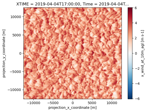
# Calculate the divergence of the flow
# Multiply by the water vapor (QVAPOR) to get the moisture divergenc

div = mpcalc.divergence(QVAPOR*ds["U10"].sel(Time=f"{case_date:%Y-%m-%d} {hour_to_plot}:00"), QVAPOR*ds["V10"].sel(Time=f"{case_date:%Y-%m-%d} {hour_to_plot}:00"))

# start figure and set axis
fig, ax = plt.subplots(figsize=(5, 5))

# plot divergence and scale by 1e5
cf = ax.contourf(ds.y, ds.x, div*1e5 , range(-15, 16, 1), cmap=plt.cm.bwr_r) #* 1e5
plt.colorbar(cf, pad=0, aspect=50)
#ax.barbs(ds.y.values, ds.x.values, ds.U10.sel(Time=f"{case_date:%Y-%m-%d} {hour_to_plot}:00"), ds.V10.sel(Time=f"{case_date:%Y-%m-%d} {hour_to_plot}:00"), color='black', length=0.5, alpha=0.5)
#ax.set(xlim=(260, 270), ylim=(30, 40))
ax.set_title('Horizontal Moisture Divergence: 10m')
#ax.set_

#plt.show()
/tmp/ipykernel_1554/326214781.py:4: UserWarning: More than one latitude coordinate present for variable .
  div = mpcalc.divergence(QVAPOR*ds["U10"].sel(Time=f"{case_date:%Y-%m-%d} {hour_to_plot}:00"), QVAPOR*ds["V10"].sel(Time=f"{case_date:%Y-%m-%d} {hour_to_plot}:00"))
Text(0.5, 1.0, 'Horizontal Moisture Divergence: 10m')
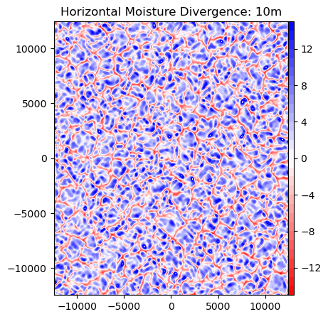
Moisture convergence at 1km
#Load in u, v, and q data
#U and V have staggered x and y dimensions. The following unstaggers them to align with QVAPOR
U = ds.U.interp(x_stag=ds.x)
V = ds.V.interp(y_stag=ds.y)

z = 1000

QVAPOR = ds["QVAPOR"].sel(z=z,method='nearest').sel(Time=f"{case_date:%Y-%m-%d} {hour_to_plot}:00")
QVAPOR.shape
(250, 250)
U_at_z = U.sel(z=z,method='nearest').sel(Time=f"{case_date:%Y-%m-%d} {hour_to_plot}:00")
V_at_z = V.sel(z=z,method='nearest').sel(Time=f"{case_date:%Y-%m-%d} {hour_to_plot}:00")

print(U_at_z.shape)
print(V_at_z.shape)
(250, 250)
(250, 250)
# Calculate the divergence of the flow
# Multiply by the water vapor (QVAPOR) to get the moisture divergenc

div2 = mpcalc.divergence(QVAPOR*U_at_z, QVAPOR*V_at_z)

# start figure and set axis
fig2, ax = plt.subplots(figsize=(5, 5))

# plot divergence and scale by 1e5
cf = ax.contourf(ds.y, ds.x, div2*1e5 , range(-15, 16, 1), cmap=plt.cm.bwr_r) #* 1e5
plt.colorbar(cf, pad=0, aspect=50)
#ax.barbs(ds.y.values, ds.x.values, ds.U10.sel(Time=f"{case_date:%Y-%m-%d} {hour_to_plot}:00"), ds.V10.sel(Time=f"{case_date:%Y-%m-%d} {hour_to_plot}:00"), color='black', length=0.5, alpha=0.5)
#ax.set(xlim=(260, 270), ylim=(30, 40))
ax.set_title('Horizontal Moisture Divergence: 1000m')


plt.show()
/tmp/ipykernel_1554/3030828318.py:4: UserWarning: More than one longitude coordinate present for variable .
  div2 = mpcalc.divergence(QVAPOR*U_at_z, QVAPOR*V_at_z)
/tmp/ipykernel_1554/3030828318.py:4: UserWarning: More than one latitude coordinate present for variable .
  div2 = mpcalc.divergence(QVAPOR*U_at_z, QVAPOR*V_at_z)
/tmp/ipykernel_1554/3030828318.py:4: UserWarning: More than one time coordinate present for variable .
  div2 = mpcalc.divergence(QVAPOR*U_at_z, QVAPOR*V_at_z)
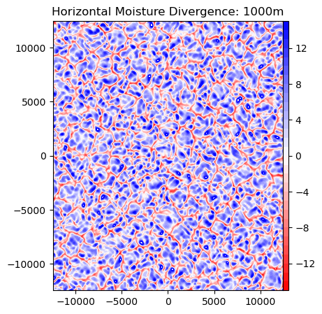
ds
<xarray.Dataset> Size: 255GB
Dimensions:                    (Time: 91, y: 250, x: 250, soil_layers_stag: 5,
                                z: 226, x_stag: 251, y_stag: 251, z_stag: 227,
                                force_layers: 751)
Coordinates: (12/15)
    CLAT                       (y, x) float32 250kB dask.array<chunksize=(125, 125), meta=np.ndarray>
    XLAT                       (y, x) float32 250kB dask.array<chunksize=(125, 125), meta=np.ndarray>
    XLONG                      (y, x) float32 250kB dask.array<chunksize=(125, 125), meta=np.ndarray>
    XTIME                      (Time) datetime64[ns] 728B dask.array<chunksize=(6,), meta=np.ndarray>
    XLAT_U                     (y, x_stag) float32 251kB dask.array<chunksize=(125, 126), meta=np.ndarray>
    XLONG_U                    (y, x_stag) float32 251kB dask.array<chunksize=(125, 126), meta=np.ndarray>
    ...                         ...
  * z_stag                     (z_stag) float32 908B 1.0 0.9959 ... 0.002178 0.0
  * Time                       (Time) datetime64[ns] 728B 2019-04-04T12:00:00...
  * y_stag                     (y_stag) float64 2kB -1.25e+04 ... 1.25e+04
  * y                          (y) float64 2kB -1.245e+04 ... 1.245e+04
  * x                          (x) float64 2kB -1.245e+04 ... 1.245e+04
  * x_stag                     (x_stag) float64 2kB -1.25e+04 ... 1.25e+04
Dimensions without coordinates: soil_layers_stag, force_layers
Data variables: (12/251)
    Times                      (Time) |S19 2kB dask.array<chunksize=(1,), meta=np.ndarray>
    LU_INDEX                   (Time, y, x) float32 23MB dask.array<chunksize=(1, 125, 125), meta=np.ndarray>
    ZS                         (Time, soil_layers_stag) float32 2kB dask.array<chunksize=(1, 5), meta=np.ndarray>
    DZS                        (Time, soil_layers_stag) float32 2kB dask.array<chunksize=(1, 5), meta=np.ndarray>
    VAR_SSO                    (Time, y, x) float32 23MB dask.array<chunksize=(1, 125, 125), meta=np.ndarray>
    U                          (Time, z, y, x_stag) float32 5GB dask.array<chunksize=(1, 226, 125, 126), meta=np.ndarray>
    ...                         ...
    geopotential               (Time, z_stag, y, x) float32 5GB dask.array<chunksize=(1, 227, 125, 125), meta=np.ndarray>
    geopotential_height        (Time, z_stag, y, x) float32 5GB dask.array<chunksize=(1, 227, 125, 125), meta=np.ndarray>
    wind_east                  (Time, z, y, x) float32 5GB dask.array<chunksize=(1, 226, 125, 125), meta=np.ndarray>
    wind_north                 (Time, z, y, x) float32 5GB dask.array<chunksize=(1, 226, 125, 125), meta=np.ndarray>
    wind_east_10               (Time, y, x) float32 23MB dask.array<chunksize=(1, 125, 125), meta=np.ndarray>
    wind_north_10              (Time, y, x) float32 23MB dask.array<chunksize=(1, 125, 125), meta=np.ndarray>
Attributes: (12/142)
    TITLE:                                  OUTPUT FROM WRF V3.8.1 MODEL
    START_DATE:                            2019-04-04_12:00:00
    SIMULATION_START_DATE:                 2019-04-04_12:00:00
    WEST-EAST_GRID_DIMENSION:              251
    SOUTH-NORTH_GRID_DIMENSION:            251
    BOTTOM-TOP_GRID_DIMENSION:             227
    ...                                    ...
    config_aerosol:                        NA
    config_forecast_time:                  15.0 h
    config_boundary_method:                Periodic
    config_microphysics:                   Thompson (mp_physics=8)
    config_nickname:                       runlas20190404v1addhm
    simulation_origin_host:                cumulus-login2.ccs.ornl.gov
xarray.Dataset
- Time: 91
- y: 250
- x: 250
- soil_layers_stag: 5
- z: 226
- x_stag: 251
- y_stag: 251
- z_stag: 227
- force_layers: 751
- CLAT(y, x)float32dask.array<chunksize=(125, 125), meta=np.ndarray>
- FieldType :
- 104
- MemoryOrder :
- XY
- description :
- COMPUTATIONAL GRID LATITUDE, SOUTH IS NEGATIVE
- units :
- degree_north
- stagger :
Array Chunk Bytes 244.14 kiB 61.04 kiB Shape (250, 250) (125, 125) Dask graph 4 chunks in 34 graph layers Data type float32 numpy.ndarray - XLAT(y, x)float32dask.array<chunksize=(125, 125), meta=np.ndarray>
- FieldType :
- 104
- MemoryOrder :
- XY
- description :
- LATITUDE, SOUTH IS NEGATIVE
- units :
- degree_north
- stagger :
Array Chunk Bytes 244.14 kiB 61.04 kiB Shape (250, 250) (125, 125) Dask graph 4 chunks in 34 graph layers Data type float32 numpy.ndarray - XLONG(y, x)float32dask.array<chunksize=(125, 125), meta=np.ndarray>
- FieldType :
- 104
- MemoryOrder :
- XY
- description :
- LONGITUDE, WEST IS NEGATIVE
- units :
- degree_east
- stagger :
Array Chunk Bytes 244.14 kiB 61.04 kiB Shape (250, 250) (125, 125) Dask graph 4 chunks in 34 graph layers Data type float32 numpy.ndarray - XTIME(Time)datetime64[ns]dask.array<chunksize=(6,), meta=np.ndarray>
- FieldType :
- 104
- MemoryOrder :
- 0
- description :
- minutes since 2019-04-04 12:00:00
- stagger :
Array Chunk Bytes 728 B 48 B Shape (91,) (6,) Dask graph 16 chunks in 33 graph layers Data type datetime64[ns] numpy.ndarray - XLAT_U(y, x_stag)float32dask.array<chunksize=(125, 126), meta=np.ndarray>
- FieldType :
- 104
- MemoryOrder :
- XY
- description :
- LATITUDE, SOUTH IS NEGATIVE
- units :
- degree_north
- stagger :
- X
Array Chunk Bytes 245.12 kiB 61.52 kiB Shape (250, 251) (125, 126) Dask graph 4 chunks in 34 graph layers Data type float32 numpy.ndarray - XLONG_U(y, x_stag)float32dask.array<chunksize=(125, 126), meta=np.ndarray>
- FieldType :
- 104
- MemoryOrder :
- XY
- description :
- LONGITUDE, WEST IS NEGATIVE
- units :
- degree_east
- stagger :
- X
Array Chunk Bytes 245.12 kiB 61.52 kiB Shape (250, 251) (125, 126) Dask graph 4 chunks in 34 graph layers Data type float32 numpy.ndarray - XLAT_V(y_stag, x)float32dask.array<chunksize=(126, 125), meta=np.ndarray>
- FieldType :
- 104
- MemoryOrder :
- XY
- description :
- LATITUDE, SOUTH IS NEGATIVE
- units :
- degree_north
- stagger :
- Y
Array Chunk Bytes 245.12 kiB 61.52 kiB Shape (251, 250) (126, 125) Dask graph 4 chunks in 34 graph layers Data type float32 numpy.ndarray - XLONG_V(y_stag, x)float32dask.array<chunksize=(126, 125), meta=np.ndarray>
- FieldType :
- 104
- MemoryOrder :
- XY
- description :
- LONGITUDE, WEST IS NEGATIVE
- units :
- degree_east
- stagger :
- Y
Array Chunk Bytes 245.12 kiB 61.52 kiB Shape (251, 250) (126, 125) Dask graph 4 chunks in 34 graph layers Data type float32 numpy.ndarray - z(z)float320.9979 0.9938 ... 0.005743 0.001089
- FieldType :
- 104
- MemoryOrder :
- Z
- description :
- eta values on half (mass) levels
- units :
- stagger :
- axis :
- Z
- standard_name :
- atmosphere_sigma_coordinate
array([0.997944, 0.993847, 0.989777, ..., 0.01304 , 0.005743, 0.001089], dtype=float32) - z_stag(z_stag)float321.0 0.9959 0.9918 ... 0.002178 0.0
- FieldType :
- 104
- MemoryOrder :
- Z
- description :
- eta values on full (w) levels
- units :
- stagger :
- Z
- axis :
- Z
- c_grid_axis_shift :
- 0.5
- standard_name :
- atmosphere_sigma_coordinate
array([1. , 0.995887, 0.991808, ..., 0.009308, 0.002178, 0. ], dtype=float32) - Time(Time)datetime64[ns]2019-04-04T12:00:00 ... 2019-04-...
- FieldType :
- 104
- MemoryOrder :
- 0
- description :
- minutes since 2019-04-04 12:00:00
- stagger :
array(['2019-04-04T12:00:00.000000000', '2019-04-04T12:10:00.000000000', '2019-04-04T12:20:00.000000000', '2019-04-04T12:30:00.000000000', '2019-04-04T12:40:00.000000000', '2019-04-04T12:50:00.000000000', '2019-04-04T13:00:00.000000000', '2019-04-04T13:10:00.000000000', '2019-04-04T13:20:00.000000000', '2019-04-04T13:30:00.000000000', '2019-04-04T13:40:00.000000000', '2019-04-04T13:50:00.000000000', '2019-04-04T14:00:00.000000000', '2019-04-04T14:10:00.000000000', '2019-04-04T14:20:00.000000000', '2019-04-04T14:30:00.000000000', '2019-04-04T14:40:00.000000000', '2019-04-04T14:50:00.000000000', '2019-04-04T15:00:00.000000000', '2019-04-04T15:10:00.000000000', '2019-04-04T15:20:00.000000000', '2019-04-04T15:30:00.000000000', '2019-04-04T15:40:00.000000000', '2019-04-04T15:50:00.000000000', '2019-04-04T16:00:00.000000000', '2019-04-04T16:10:00.000000000', '2019-04-04T16:20:00.000000000', '2019-04-04T16:30:00.000000000', '2019-04-04T16:40:00.000000000', '2019-04-04T16:50:00.000000000', '2019-04-04T17:00:00.000000000', '2019-04-04T17:10:00.000000000', '2019-04-04T17:20:00.000000000', '2019-04-04T17:30:00.000000000', '2019-04-04T17:40:00.000000000', '2019-04-04T17:50:00.000000000', '2019-04-04T18:00:00.000000000', '2019-04-04T18:10:00.000000000', '2019-04-04T18:20:00.000000000', '2019-04-04T18:30:00.000000000', '2019-04-04T18:40:00.000000000', '2019-04-04T18:50:00.000000000', '2019-04-04T19:00:00.000000000', '2019-04-04T19:10:00.000000000', '2019-04-04T19:20:00.000000000', '2019-04-04T19:30:00.000000000', '2019-04-04T19:40:00.000000000', '2019-04-04T19:50:00.000000000', '2019-04-04T20:00:00.000000000', '2019-04-04T20:10:00.000000000', '2019-04-04T20:20:00.000000000', '2019-04-04T20:30:00.000000000', '2019-04-04T20:40:00.000000000', '2019-04-04T20:50:00.000000000', '2019-04-04T21:00:00.000000000', '2019-04-04T21:10:00.000000000', '2019-04-04T21:20:00.000000000', '2019-04-04T21:30:00.000000000', '2019-04-04T21:40:00.000000000', '2019-04-04T21:50:00.000000000', '2019-04-04T22:00:00.000000000', '2019-04-04T22:10:00.000000000', '2019-04-04T22:20:00.000000000', '2019-04-04T22:30:00.000000000', '2019-04-04T22:40:00.000000000', '2019-04-04T22:50:00.000000000', '2019-04-04T23:00:00.000000000', '2019-04-04T23:10:00.000000000', '2019-04-04T23:20:00.000000000', '2019-04-04T23:30:00.000000000', '2019-04-04T23:40:00.000000000', '2019-04-04T23:50:00.000000000', '2019-04-05T00:00:00.000000000', '2019-04-05T00:10:00.000000000', '2019-04-05T00:20:00.000000000', '2019-04-05T00:30:00.000000000', '2019-04-05T00:40:00.000000000', '2019-04-05T00:50:00.000000000', '2019-04-05T01:00:00.000000000', '2019-04-05T01:10:00.000000000', '2019-04-05T01:20:00.000000000', '2019-04-05T01:30:00.000000000', '2019-04-05T01:40:00.000000000', '2019-04-05T01:50:00.000000000', '2019-04-05T02:00:00.000000000', '2019-04-05T02:10:00.000000000', '2019-04-05T02:20:00.000000000', '2019-04-05T02:30:00.000000000', '2019-04-05T02:40:00.000000000', '2019-04-05T02:50:00.000000000', '2019-04-05T03:00:00.000000000'], dtype='datetime64[ns]') - y_stag(y_stag)float64-1.25e+04 -1.24e+04 ... 1.25e+04
- units :
- m
- standard_name :
- projection_y_coordinate
- axis :
- Y
- c_grid_axis_shift :
- 0.5
array([-12500., -12400., -12300., ..., 12300., 12400., 12500.])
- y(y)float64-1.245e+04 -1.235e+04 ... 1.245e+04
- units :
- m
- standard_name :
- projection_y_coordinate
- axis :
- Y
array([-12450., -12350., -12250., ..., 12250., 12350., 12450.])
- x(x)float64-1.245e+04 -1.235e+04 ... 1.245e+04
- units :
- m
- standard_name :
- projection_x_coordinate
- axis :
- X
array([-12450., -12350., -12250., ..., 12250., 12350., 12450.])
- x_stag(x_stag)float64-1.25e+04 -1.24e+04 ... 1.25e+04
- units :
- m
- standard_name :
- projection_x_coordinate
- axis :
- X
- c_grid_axis_shift :
- 0.5
array([-12500., -12400., -12300., ..., 12300., 12400., 12500.])
- Times(Time)|S19dask.array<chunksize=(1,), meta=np.ndarray>
Array Chunk Bytes 1.69 kiB 19 B Shape (91,) (1,) Dask graph 91 chunks in 33 graph layers Data type |S19 numpy.ndarray - LU_INDEX(Time, y, x)float32dask.array<chunksize=(1, 125, 125), meta=np.ndarray>
- FieldType :
- 104
- MemoryOrder :
- XY
- description :
- LAND USE CATEGORY
- units :
- stagger :
Array Chunk Bytes 21.70 MiB 61.04 kiB Shape (91, 250, 250) (1, 125, 125) Dask graph 364 chunks in 33 graph layers Data type float32 numpy.ndarray - ZS(Time, soil_layers_stag)float32dask.array<chunksize=(1, 5), meta=np.ndarray>
- FieldType :
- 104
- MemoryOrder :
- Z
- description :
- DEPTHS OF CENTERS OF SOIL LAYERS
- units :
- m
- stagger :
- Z
Array Chunk Bytes 1.78 kiB 20 B Shape (91, 5) (1, 5) Dask graph 91 chunks in 33 graph layers Data type float32 numpy.ndarray - DZS(Time, soil_layers_stag)float32dask.array<chunksize=(1, 5), meta=np.ndarray>
- FieldType :
- 104
- MemoryOrder :
- Z
- description :
- THICKNESSES OF SOIL LAYERS
- units :
- m
- stagger :
- Z
Array Chunk Bytes 1.78 kiB 20 B Shape (91, 5) (1, 5) Dask graph 91 chunks in 33 graph layers Data type float32 numpy.ndarray - VAR_SSO(Time, y, x)float32dask.array<chunksize=(1, 125, 125), meta=np.ndarray>
- FieldType :
- 104
- MemoryOrder :
- XY
- description :
- Variance of Subgrid Scale Orography MSL
- units :
- m2
- stagger :
Array Chunk Bytes 21.70 MiB 61.04 kiB Shape (91, 250, 250) (1, 125, 125) Dask graph 364 chunks in 33 graph layers Data type float32 numpy.ndarray - U(Time, z, y, x_stag)float32dask.array<chunksize=(1, 226, 125, 126), meta=np.ndarray>
- FieldType :
- 104
- MemoryOrder :
- XYZ
- description :
- x-wind component
- units :
- m s-1
- stagger :
- X
- standard_name :
- x_wind
Array Chunk Bytes 4.81 GiB 13.58 MiB Shape (91, 226, 250, 251) (1, 226, 125, 126) Dask graph 364 chunks in 33 graph layers Data type float32 numpy.ndarray - V(Time, z, y_stag, x)float32dask.array<chunksize=(1, 226, 126, 125), meta=np.ndarray>
- FieldType :
- 104
- MemoryOrder :
- XYZ
- description :
- y-wind component
- units :
- m s-1
- stagger :
- Y
- standard_name :
- y_wind
Array Chunk Bytes 4.81 GiB 13.58 MiB Shape (91, 226, 251, 250) (1, 226, 126, 125) Dask graph 364 chunks in 33 graph layers Data type float32 numpy.ndarray - W(Time, z_stag, y, x)float32dask.array<chunksize=(1, 227, 125, 125), meta=np.ndarray>
- FieldType :
- 104
- MemoryOrder :
- XYZ
- description :
- z-wind component
- units :
- m s-1
- stagger :
- Z
- standard_name :
- upward_air_velocity
Array Chunk Bytes 4.81 GiB 13.53 MiB Shape (91, 227, 250, 250) (1, 227, 125, 125) Dask graph 364 chunks in 33 graph layers Data type float32 numpy.ndarray - HFX_FORCE(Time)float32dask.array<chunksize=(6,), meta=np.ndarray>
- FieldType :
- 104
- MemoryOrder :
- 0
- description :
- SCM ideal surface sensible heat flux
- units :
- W m-2
- stagger :
Array Chunk Bytes 364 B 24 B Shape (91,) (6,) Dask graph 16 chunks in 33 graph layers Data type float32 numpy.ndarray - LH_FORCE(Time)float32dask.array<chunksize=(6,), meta=np.ndarray>
- FieldType :
- 104
- MemoryOrder :
- 0
- description :
- SCM ideal surface latent heat flux
- units :
- W m-2
- stagger :
Array Chunk Bytes 364 B 24 B Shape (91,) (6,) Dask graph 16 chunks in 33 graph layers Data type float32 numpy.ndarray - TSK_FORCE(Time)float32dask.array<chunksize=(6,), meta=np.ndarray>
- FieldType :
- 104
- MemoryOrder :
- 0
- description :
- SCM ideal surface skin temperature
- units :
- W m-2
- stagger :
Array Chunk Bytes 364 B 24 B Shape (91,) (6,) Dask graph 16 chunks in 33 graph layers Data type float32 numpy.ndarray - HFX_FORCE_TEND(Time)float32dask.array<chunksize=(6,), meta=np.ndarray>
- FieldType :
- 104
- MemoryOrder :
- 0
- description :
- SCM ideal surface sensible heat flux tendency
- units :
- W m-2 s-1
- stagger :
Array Chunk Bytes 364 B 24 B Shape (91,) (6,) Dask graph 16 chunks in 33 graph layers Data type float32 numpy.ndarray - LH_FORCE_TEND(Time)float32dask.array<chunksize=(6,), meta=np.ndarray>
- FieldType :
- 104
- MemoryOrder :
- 0
- description :
- SCM ideal surface latent heat flux tendency
- units :
- W m-2 s-1
- stagger :
Array Chunk Bytes 364 B 24 B Shape (91,) (6,) Dask graph 16 chunks in 33 graph layers Data type float32 numpy.ndarray - TSK_FORCE_TEND(Time)float32dask.array<chunksize=(6,), meta=np.ndarray>
- FieldType :
- 104
- MemoryOrder :
- 0
- description :
- SCM ideal surface skin temperature tendency
- units :
- W m-2 s-1
- stagger :
Array Chunk Bytes 364 B 24 B Shape (91,) (6,) Dask graph 16 chunks in 33 graph layers Data type float32 numpy.ndarray - MU(Time, y, x)float32dask.array<chunksize=(1, 125, 125), meta=np.ndarray>
- FieldType :
- 104
- MemoryOrder :
- XY
- description :
- perturbation dry air mass in column
- units :
- Pa
- stagger :
Array Chunk Bytes 21.70 MiB 61.04 kiB Shape (91, 250, 250) (1, 125, 125) Dask graph 364 chunks in 33 graph layers Data type float32 numpy.ndarray - MUB(Time, y, x)float32dask.array<chunksize=(1, 125, 125), meta=np.ndarray>
- FieldType :
- 104
- MemoryOrder :
- XY
- description :
- base state dry air mass in column
- units :
- Pa
- stagger :
Array Chunk Bytes 21.70 MiB 61.04 kiB Shape (91, 250, 250) (1, 125, 125) Dask graph 364 chunks in 33 graph layers Data type float32 numpy.ndarray - NEST_POS(Time, y, x)float32dask.array<chunksize=(1, 125, 125), meta=np.ndarray>
- FieldType :
- 104
- MemoryOrder :
- XY
- description :
- -
- stagger :
Array Chunk Bytes 21.70 MiB 61.04 kiB Shape (91, 250, 250) (1, 125, 125) Dask graph 364 chunks in 33 graph layers Data type float32 numpy.ndarray - TKE(Time, z, y, x)float32dask.array<chunksize=(1, 226, 125, 125), meta=np.ndarray>
- FieldType :
- 104
- MemoryOrder :
- XYZ
- description :
- TURBULENCE KINETIC ENERGY
- units :
- m2 s-2
- stagger :
Array Chunk Bytes 4.79 GiB 13.47 MiB Shape (91, 226, 250, 250) (1, 226, 125, 125) Dask graph 364 chunks in 33 graph layers Data type float32 numpy.ndarray - ALT(Time, z, y, x)float32dask.array<chunksize=(1, 226, 125, 125), meta=np.ndarray>
- FieldType :
- 104
- MemoryOrder :
- XYZ
- description :
- inverse density
- units :
- m3 kg-1
- stagger :
Array Chunk Bytes 4.79 GiB 13.47 MiB Shape (91, 226, 250, 250) (1, 226, 125, 125) Dask graph 364 chunks in 33 graph layers Data type float32 numpy.ndarray - FNM(Time, z)float32dask.array<chunksize=(1, 226), meta=np.ndarray>
- FieldType :
- 104
- MemoryOrder :
- Z
- description :
- upper weight for vertical stretching
- units :
- stagger :
Array Chunk Bytes 80.34 kiB 904 B Shape (91, 226) (1, 226) Dask graph 91 chunks in 33 graph layers Data type float32 numpy.ndarray - FNP(Time, z)float32dask.array<chunksize=(1, 226), meta=np.ndarray>
- FieldType :
- 104
- MemoryOrder :
- Z
- description :
- lower weight for vertical stretching
- units :
- stagger :
Array Chunk Bytes 80.34 kiB 904 B Shape (91, 226) (1, 226) Dask graph 91 chunks in 33 graph layers Data type float32 numpy.ndarray - RDNW(Time, z)float32dask.array<chunksize=(1, 226), meta=np.ndarray>
- FieldType :
- 104
- MemoryOrder :
- Z
- description :
- inverse d(eta) values between full (w) levels
- units :
- stagger :
Array Chunk Bytes 80.34 kiB 904 B Shape (91, 226) (1, 226) Dask graph 91 chunks in 33 graph layers Data type float32 numpy.ndarray - RDN(Time, z)float32dask.array<chunksize=(1, 226), meta=np.ndarray>
- FieldType :
- 104
- MemoryOrder :
- Z
- description :
- inverse d(eta) values between half (mass) levels
- units :
- stagger :
Array Chunk Bytes 80.34 kiB 904 B Shape (91, 226) (1, 226) Dask graph 91 chunks in 33 graph layers Data type float32 numpy.ndarray - DNW(Time, z)float32dask.array<chunksize=(1, 226), meta=np.ndarray>
- FieldType :
- 104
- MemoryOrder :
- Z
- description :
- d(eta) values between full (w) levels
- units :
- stagger :
Array Chunk Bytes 80.34 kiB 904 B Shape (91, 226) (1, 226) Dask graph 91 chunks in 33 graph layers Data type float32 numpy.ndarray - DN(Time, z)float32dask.array<chunksize=(1, 226), meta=np.ndarray>
- FieldType :
- 104
- MemoryOrder :
- Z
- description :
- d(eta) values between half (mass) levels
- units :
- stagger :
Array Chunk Bytes 80.34 kiB 904 B Shape (91, 226) (1, 226) Dask graph 91 chunks in 33 graph layers Data type float32 numpy.ndarray - CFN(Time)float32dask.array<chunksize=(6,), meta=np.ndarray>
- FieldType :
- 104
- MemoryOrder :
- 0
- description :
- extrapolation constant
- units :
- stagger :
Array Chunk Bytes 364 B 24 B Shape (91,) (6,) Dask graph 16 chunks in 33 graph layers Data type float32 numpy.ndarray - CFN1(Time)float32dask.array<chunksize=(6,), meta=np.ndarray>
- FieldType :
- 104
- MemoryOrder :
- 0
- description :
- extrapolation constant
- units :
- stagger :
Array Chunk Bytes 364 B 24 B Shape (91,) (6,) Dask graph 16 chunks in 33 graph layers Data type float32 numpy.ndarray - THIS_IS_AN_IDEAL_RUN(Time)int32dask.array<chunksize=(6,), meta=np.ndarray>
- FieldType :
- 106
- MemoryOrder :
- 0
- description :
- T/F flag: this is an ARW ideal simulation
- stagger :
Array Chunk Bytes 364 B 24 B Shape (91,) (6,) Dask graph 16 chunks in 33 graph layers Data type int32 numpy.ndarray - P_HYD(Time, z, y, x)float32dask.array<chunksize=(1, 226, 125, 125), meta=np.ndarray>
- FieldType :
- 104
- MemoryOrder :
- XYZ
- description :
- hydrostatic pressure
- units :
- Pa
- stagger :
Array Chunk Bytes 4.79 GiB 13.47 MiB Shape (91, 226, 250, 250) (1, 226, 125, 125) Dask graph 364 chunks in 33 graph layers Data type float32 numpy.ndarray - Q2(Time, y, x)float32dask.array<chunksize=(1, 125, 125), meta=np.ndarray>
- FieldType :
- 104
- MemoryOrder :
- XY
- description :
- QV at 2 M
- units :
- kg kg-1
- stagger :
- standard_name :
- humidity_mixing_ratio
- long_name :
- humidity_mixing_ratio_at_2m_agl
Array Chunk Bytes 21.70 MiB 61.04 kiB Shape (91, 250, 250) (1, 125, 125) Dask graph 364 chunks in 33 graph layers Data type float32 numpy.ndarray - T2(Time, y, x)float32dask.array<chunksize=(1, 125, 125), meta=np.ndarray>
- FieldType :
- 104
- MemoryOrder :
- XY
- description :
- TEMP at 2 M
- units :
- K
- stagger :
- standard_name :
- air_temperature
- long_name :
- air_temperature_at_2m_agl
Array Chunk Bytes 21.70 MiB 61.04 kiB Shape (91, 250, 250) (1, 125, 125) Dask graph 364 chunks in 33 graph layers Data type float32 numpy.ndarray - TH2(Time, y, x)float32dask.array<chunksize=(1, 125, 125), meta=np.ndarray>
- FieldType :
- 104
- MemoryOrder :
- XY
- description :
- POT TEMP at 2 M
- units :
- K
- stagger :
- standard_name :
- air_potential_temperature
- long_name :
- air_potential_temperature_at_2m_agl
Array Chunk Bytes 21.70 MiB 61.04 kiB Shape (91, 250, 250) (1, 125, 125) Dask graph 364 chunks in 33 graph layers Data type float32 numpy.ndarray - PSFC(Time, y, x)float32dask.array<chunksize=(1, 125, 125), meta=np.ndarray>
- FieldType :
- 104
- MemoryOrder :
- XY
- description :
- SFC PRESSURE
- units :
- Pa
- stagger :
- standard_name :
- air_pressure
- long_name :
- air_pressure_at_surface
Array Chunk Bytes 21.70 MiB 61.04 kiB Shape (91, 250, 250) (1, 125, 125) Dask graph 364 chunks in 33 graph layers Data type float32 numpy.ndarray - U10(Time, y, x)float32dask.array<chunksize=(1, 125, 125), meta=np.ndarray>
- FieldType :
- 104
- MemoryOrder :
- XY
- description :
- U at 10 M
- units :
- m s-1
- stagger :
- standard_name :
- x_wind
- long_name :
- x_wind_at_10m_agl
Array Chunk Bytes 21.70 MiB 61.04 kiB Shape (91, 250, 250) (1, 125, 125) Dask graph 364 chunks in 33 graph layers Data type float32 numpy.ndarray - V10(Time, y, x)float32dask.array<chunksize=(1, 125, 125), meta=np.ndarray>
- FieldType :
- 104
- MemoryOrder :
- XY
- description :
- V at 10 M
- units :
- m s-1
- stagger :
- standard_name :
- y_wind
- long_name :
- y_wind_at_10m_agl
Array Chunk Bytes 21.70 MiB 61.04 kiB Shape (91, 250, 250) (1, 125, 125) Dask graph 364 chunks in 33 graph layers Data type float32 numpy.ndarray - RDX(Time)float32dask.array<chunksize=(6,), meta=np.ndarray>
- FieldType :
- 104
- MemoryOrder :
- 0
- description :
- INVERSE X GRID LENGTH
- units :
- stagger :
Array Chunk Bytes 364 B 24 B Shape (91,) (6,) Dask graph 16 chunks in 33 graph layers Data type float32 numpy.ndarray - RDY(Time)float32dask.array<chunksize=(6,), meta=np.ndarray>
- FieldType :
- 104
- MemoryOrder :
- 0
- description :
- INVERSE Y GRID LENGTH
- units :
- stagger :
Array Chunk Bytes 364 B 24 B Shape (91,) (6,) Dask graph 16 chunks in 33 graph layers Data type float32 numpy.ndarray - RESM(Time)float32dask.array<chunksize=(6,), meta=np.ndarray>
- FieldType :
- 104
- MemoryOrder :
- 0
- description :
- TIME WEIGHT CONSTANT FOR SMALL STEPS
- units :
- stagger :
Array Chunk Bytes 364 B 24 B Shape (91,) (6,) Dask graph 16 chunks in 33 graph layers Data type float32 numpy.ndarray - ZETATOP(Time)float32dask.array<chunksize=(6,), meta=np.ndarray>
- FieldType :
- 104
- MemoryOrder :
- 0
- description :
- ZETA AT MODEL TOP
- units :
- stagger :
Array Chunk Bytes 364 B 24 B Shape (91,) (6,) Dask graph 16 chunks in 33 graph layers Data type float32 numpy.ndarray - CF1(Time)float32dask.array<chunksize=(6,), meta=np.ndarray>
- FieldType :
- 104
- MemoryOrder :
- 0
- description :
- 2nd order extrapolation constant
- units :
- stagger :
Array Chunk Bytes 364 B 24 B Shape (91,) (6,) Dask graph 16 chunks in 33 graph layers Data type float32 numpy.ndarray - CF2(Time)float32dask.array<chunksize=(6,), meta=np.ndarray>
- FieldType :
- 104
- MemoryOrder :
- 0
- description :
- 2nd order extrapolation constant
- units :
- stagger :
Array Chunk Bytes 364 B 24 B Shape (91,) (6,) Dask graph 16 chunks in 33 graph layers Data type float32 numpy.ndarray - CF3(Time)float32dask.array<chunksize=(6,), meta=np.ndarray>
- FieldType :
- 104
- MemoryOrder :
- 0
- description :
- 2nd order extrapolation constant
- units :
- stagger :
Array Chunk Bytes 364 B 24 B Shape (91,) (6,) Dask graph 16 chunks in 33 graph layers Data type float32 numpy.ndarray - ITIMESTEP(Time)int32dask.array<chunksize=(6,), meta=np.ndarray>
- FieldType :
- 106
- MemoryOrder :
- 0
- description :
- units :
- stagger :
Array Chunk Bytes 364 B 24 B Shape (91,) (6,) Dask graph 16 chunks in 33 graph layers Data type int32 numpy.ndarray - QVAPOR(Time, z, y, x)float32dask.array<chunksize=(1, 226, 125, 125), meta=np.ndarray>
- FieldType :
- 104
- MemoryOrder :
- XYZ
- description :
- Water vapor mixing ratio
- units :
- kg kg-1
- stagger :
- standard_name :
- humidity_mixing_ratio
Array Chunk Bytes 4.79 GiB 13.47 MiB Shape (91, 226, 250, 250) (1, 226, 125, 125) Dask graph 364 chunks in 33 graph layers Data type float32 numpy.ndarray - QCLOUD(Time, z, y, x)float32dask.array<chunksize=(1, 226, 125, 125), meta=np.ndarray>
- FieldType :
- 104
- MemoryOrder :
- XYZ
- description :
- Cloud water mixing ratio
- units :
- kg kg-1
- stagger :
Array Chunk Bytes 4.79 GiB 13.47 MiB Shape (91, 226, 250, 250) (1, 226, 125, 125) Dask graph 364 chunks in 33 graph layers Data type float32 numpy.ndarray - QRAIN(Time, z, y, x)float32dask.array<chunksize=(1, 226, 125, 125), meta=np.ndarray>
- FieldType :
- 104
- MemoryOrder :
- XYZ
- description :
- Rain water mixing ratio
- units :
- kg kg-1
- stagger :
Array Chunk Bytes 4.79 GiB 13.47 MiB Shape (91, 226, 250, 250) (1, 226, 125, 125) Dask graph 364 chunks in 33 graph layers Data type float32 numpy.ndarray - QICE(Time, z, y, x)float32dask.array<chunksize=(1, 226, 125, 125), meta=np.ndarray>
- FieldType :
- 104
- MemoryOrder :
- XYZ
- description :
- Ice mixing ratio
- units :
- kg kg-1
- stagger :
Array Chunk Bytes 4.79 GiB 13.47 MiB Shape (91, 226, 250, 250) (1, 226, 125, 125) Dask graph 364 chunks in 33 graph layers Data type float32 numpy.ndarray - QSNOW(Time, z, y, x)float32dask.array<chunksize=(1, 226, 125, 125), meta=np.ndarray>
- FieldType :
- 104
- MemoryOrder :
- XYZ
- description :
- Snow mixing ratio
- units :
- kg kg-1
- stagger :
Array Chunk Bytes 4.79 GiB 13.47 MiB Shape (91, 226, 250, 250) (1, 226, 125, 125) Dask graph 364 chunks in 33 graph layers Data type float32 numpy.ndarray - QGRAUP(Time, z, y, x)float32dask.array<chunksize=(1, 226, 125, 125), meta=np.ndarray>
- FieldType :
- 104
- MemoryOrder :
- XYZ
- description :
- Graupel mixing ratio
- units :
- kg kg-1
- stagger :
Array Chunk Bytes 4.79 GiB 13.47 MiB Shape (91, 226, 250, 250) (1, 226, 125, 125) Dask graph 364 chunks in 33 graph layers Data type float32 numpy.ndarray - QNICE(Time, z, y, x)float32dask.array<chunksize=(1, 226, 125, 125), meta=np.ndarray>
- FieldType :
- 104
- MemoryOrder :
- XYZ
- description :
- Ice Number concentration
- units :
- kg-1
- stagger :
Array Chunk Bytes 4.79 GiB 13.47 MiB Shape (91, 226, 250, 250) (1, 226, 125, 125) Dask graph 364 chunks in 33 graph layers Data type float32 numpy.ndarray - QNRAIN(Time, z, y, x)float32dask.array<chunksize=(1, 226, 125, 125), meta=np.ndarray>
- FieldType :
- 104
- MemoryOrder :
- XYZ
- description :
- Rain Number concentration
- units :
- kg-1
- stagger :
Array Chunk Bytes 4.79 GiB 13.47 MiB Shape (91, 226, 250, 250) (1, 226, 125, 125) Dask graph 364 chunks in 33 graph layers Data type float32 numpy.ndarray - SHDMAX(Time, y, x)float32dask.array<chunksize=(1, 125, 125), meta=np.ndarray>
- FieldType :
- 104
- MemoryOrder :
- XY
- description :
- ANNUAL MAX VEG FRACTION
- units :
- stagger :
Array Chunk Bytes 21.70 MiB 61.04 kiB Shape (91, 250, 250) (1, 125, 125) Dask graph 364 chunks in 33 graph layers Data type float32 numpy.ndarray - SHDMIN(Time, y, x)float32dask.array<chunksize=(1, 125, 125), meta=np.ndarray>
- FieldType :
- 104
- MemoryOrder :
- XY
- description :
- ANNUAL MIN VEG FRACTION
- units :
- stagger :
Array Chunk Bytes 21.70 MiB 61.04 kiB Shape (91, 250, 250) (1, 125, 125) Dask graph 364 chunks in 33 graph layers Data type float32 numpy.ndarray - SNOALB(Time, y, x)float32dask.array<chunksize=(1, 125, 125), meta=np.ndarray>
- FieldType :
- 104
- MemoryOrder :
- XY
- description :
- ANNUAL MAX SNOW ALBEDO IN FRACTION
- units :
- stagger :
Array Chunk Bytes 21.70 MiB 61.04 kiB Shape (91, 250, 250) (1, 125, 125) Dask graph 364 chunks in 33 graph layers Data type float32 numpy.ndarray - TSLB(Time, soil_layers_stag, y, x)float32dask.array<chunksize=(1, 5, 125, 125), meta=np.ndarray>
- FieldType :
- 104
- MemoryOrder :
- XYZ
- description :
- SOIL TEMPERATURE
- units :
- K
- stagger :
- Z
Array Chunk Bytes 108.48 MiB 305.18 kiB Shape (91, 5, 250, 250) (1, 5, 125, 125) Dask graph 364 chunks in 33 graph layers Data type float32 numpy.ndarray - SMOIS(Time, soil_layers_stag, y, x)float32dask.array<chunksize=(1, 5, 125, 125), meta=np.ndarray>
- FieldType :
- 104
- MemoryOrder :
- XYZ
- description :
- SOIL MOISTURE
- units :
- m3 m-3
- stagger :
- Z
Array Chunk Bytes 108.48 MiB 305.18 kiB Shape (91, 5, 250, 250) (1, 5, 125, 125) Dask graph 364 chunks in 33 graph layers Data type float32 numpy.ndarray - SH2O(Time, soil_layers_stag, y, x)float32dask.array<chunksize=(1, 5, 125, 125), meta=np.ndarray>
- FieldType :
- 104
- MemoryOrder :
- XYZ
- description :
- SOIL LIQUID WATER
- units :
- m3 m-3
- stagger :
- Z
Array Chunk Bytes 108.48 MiB 305.18 kiB Shape (91, 5, 250, 250) (1, 5, 125, 125) Dask graph 364 chunks in 33 graph layers Data type float32 numpy.ndarray - SEAICE(Time, y, x)float32dask.array<chunksize=(1, 125, 125), meta=np.ndarray>
- FieldType :
- 104
- MemoryOrder :
- XY
- description :
- SEA ICE FLAG
- units :
- stagger :
Array Chunk Bytes 21.70 MiB 61.04 kiB Shape (91, 250, 250) (1, 125, 125) Dask graph 364 chunks in 33 graph layers Data type float32 numpy.ndarray - XICEM(Time, y, x)float32dask.array<chunksize=(1, 125, 125), meta=np.ndarray>
- FieldType :
- 104
- MemoryOrder :
- XY
- description :
- SEA ICE FLAG (PREVIOUS STEP)
- units :
- stagger :
Array Chunk Bytes 21.70 MiB 61.04 kiB Shape (91, 250, 250) (1, 125, 125) Dask graph 364 chunks in 33 graph layers Data type float32 numpy.ndarray - SFROFF(Time, y, x)float32dask.array<chunksize=(1, 125, 125), meta=np.ndarray>
- FieldType :
- 104
- MemoryOrder :
- XY
- description :
- SURFACE RUNOFF
- units :
- mm
- stagger :
Array Chunk Bytes 21.70 MiB 61.04 kiB Shape (91, 250, 250) (1, 125, 125) Dask graph 364 chunks in 33 graph layers Data type float32 numpy.ndarray - UDROFF(Time, y, x)float32dask.array<chunksize=(1, 125, 125), meta=np.ndarray>
- FieldType :
- 104
- MemoryOrder :
- XY
- description :
- UNDERGROUND RUNOFF
- units :
- mm
- stagger :
Array Chunk Bytes 21.70 MiB 61.04 kiB Shape (91, 250, 250) (1, 125, 125) Dask graph 364 chunks in 33 graph layers Data type float32 numpy.ndarray - IVGTYP(Time, y, x)int32dask.array<chunksize=(1, 125, 125), meta=np.ndarray>
- FieldType :
- 106
- MemoryOrder :
- XY
- description :
- DOMINANT VEGETATION CATEGORY
- units :
- stagger :
Array Chunk Bytes 21.70 MiB 61.04 kiB Shape (91, 250, 250) (1, 125, 125) Dask graph 364 chunks in 33 graph layers Data type int32 numpy.ndarray - ISLTYP(Time, y, x)int32dask.array<chunksize=(1, 125, 125), meta=np.ndarray>
- FieldType :
- 106
- MemoryOrder :
- XY
- description :
- DOMINANT SOIL CATEGORY
- units :
- stagger :
Array Chunk Bytes 21.70 MiB 61.04 kiB Shape (91, 250, 250) (1, 125, 125) Dask graph 364 chunks in 33 graph layers Data type int32 numpy.ndarray - VEGFRA(Time, y, x)float32dask.array<chunksize=(1, 125, 125), meta=np.ndarray>
- FieldType :
- 104
- MemoryOrder :
- XY
- description :
- VEGETATION FRACTION
- units :
- stagger :
- standard_name :
- vegetation_area_fraction
Array Chunk Bytes 21.70 MiB 61.04 kiB Shape (91, 250, 250) (1, 125, 125) Dask graph 364 chunks in 33 graph layers Data type float32 numpy.ndarray - GRDFLX(Time, y, x)float32dask.array<chunksize=(1, 125, 125), meta=np.ndarray>
- FieldType :
- 104
- MemoryOrder :
- XY
- description :
- GROUND HEAT FLUX
- units :
- W m-2
- stagger :
Array Chunk Bytes 21.70 MiB 61.04 kiB Shape (91, 250, 250) (1, 125, 125) Dask graph 364 chunks in 33 graph layers Data type float32 numpy.ndarray - ACGRDFLX(Time, y, x)float32dask.array<chunksize=(1, 125, 125), meta=np.ndarray>
- FieldType :
- 104
- MemoryOrder :
- XY
- description :
- ACCUMULATED GROUND HEAT FLUX
- units :
- J m-2
- stagger :
Array Chunk Bytes 21.70 MiB 61.04 kiB Shape (91, 250, 250) (1, 125, 125) Dask graph 364 chunks in 33 graph layers Data type float32 numpy.ndarray - ACSNOM(Time, y, x)float32dask.array<chunksize=(1, 125, 125), meta=np.ndarray>
- FieldType :
- 104
- MemoryOrder :
- XY
- description :
- ACCUMULATED MELTED SNOW
- units :
- kg m-2
- stagger :
Array Chunk Bytes 21.70 MiB 61.04 kiB Shape (91, 250, 250) (1, 125, 125) Dask graph 364 chunks in 33 graph layers Data type float32 numpy.ndarray - SNOW(Time, y, x)float32dask.array<chunksize=(1, 125, 125), meta=np.ndarray>
- FieldType :
- 104
- MemoryOrder :
- XY
- description :
- SNOW WATER EQUIVALENT
- units :
- kg m-2
- stagger :
Array Chunk Bytes 21.70 MiB 61.04 kiB Shape (91, 250, 250) (1, 125, 125) Dask graph 364 chunks in 33 graph layers Data type float32 numpy.ndarray - SNOWH(Time, y, x)float32dask.array<chunksize=(1, 125, 125), meta=np.ndarray>
- FieldType :
- 104
- MemoryOrder :
- XY
- description :
- PHYSICAL SNOW DEPTH
- units :
- m
- stagger :
Array Chunk Bytes 21.70 MiB 61.04 kiB Shape (91, 250, 250) (1, 125, 125) Dask graph 364 chunks in 33 graph layers Data type float32 numpy.ndarray - CANWAT(Time, y, x)float32dask.array<chunksize=(1, 125, 125), meta=np.ndarray>
- FieldType :
- 104
- MemoryOrder :
- XY
- description :
- CANOPY WATER
- units :
- kg m-2
- stagger :
Array Chunk Bytes 21.70 MiB 61.04 kiB Shape (91, 250, 250) (1, 125, 125) Dask graph 364 chunks in 33 graph layers Data type float32 numpy.ndarray - SSTSK(Time, y, x)float32dask.array<chunksize=(1, 125, 125), meta=np.ndarray>
- FieldType :
- 104
- MemoryOrder :
- XY
- description :
- SKIN SEA SURFACE TEMPERATURE
- units :
- K
- stagger :
Array Chunk Bytes 21.70 MiB 61.04 kiB Shape (91, 250, 250) (1, 125, 125) Dask graph 364 chunks in 33 graph layers Data type float32 numpy.ndarray - COSZEN(Time, y, x)float32dask.array<chunksize=(1, 125, 125), meta=np.ndarray>
- FieldType :
- 104
- MemoryOrder :
- XY
- description :
- COS of SOLAR ZENITH ANGLE
- units :
- 1
- stagger :
Array Chunk Bytes 21.70 MiB 61.04 kiB Shape (91, 250, 250) (1, 125, 125) Dask graph 364 chunks in 33 graph layers Data type float32 numpy.ndarray - LAI(Time, y, x)float32dask.array<chunksize=(1, 125, 125), meta=np.ndarray>
- FieldType :
- 104
- MemoryOrder :
- XY
- description :
- LEAF AREA INDEX
- units :
- m-2/m-2
- stagger :
- standard_name :
- leaf_area_index
Array Chunk Bytes 21.70 MiB 61.04 kiB Shape (91, 250, 250) (1, 125, 125) Dask graph 364 chunks in 33 graph layers Data type float32 numpy.ndarray - VAR(Time, y, x)float32dask.array<chunksize=(1, 125, 125), meta=np.ndarray>
- FieldType :
- 104
- MemoryOrder :
- XY
- description :
- OROGRAPHIC VARIANCE
- units :
- stagger :
Array Chunk Bytes 21.70 MiB 61.04 kiB Shape (91, 250, 250) (1, 125, 125) Dask graph 364 chunks in 33 graph layers Data type float32 numpy.ndarray - MAPFAC_M(Time, y, x)float32dask.array<chunksize=(1, 125, 125), meta=np.ndarray>
- FieldType :
- 104
- MemoryOrder :
- XY
- description :
- Map scale factor on mass grid
- units :
- stagger :
Array Chunk Bytes 21.70 MiB 61.04 kiB Shape (91, 250, 250) (1, 125, 125) Dask graph 364 chunks in 33 graph layers Data type float32 numpy.ndarray - MAPFAC_U(Time, y, x_stag)float32dask.array<chunksize=(1, 125, 126), meta=np.ndarray>
- FieldType :
- 104
- MemoryOrder :
- XY
- description :
- Map scale factor on u-grid
- units :
- stagger :
- X
Array Chunk Bytes 21.78 MiB 61.52 kiB Shape (91, 250, 251) (1, 125, 126) Dask graph 364 chunks in 33 graph layers Data type float32 numpy.ndarray - MAPFAC_V(Time, y_stag, x)float32dask.array<chunksize=(1, 126, 125), meta=np.ndarray>
- FieldType :
- 104
- MemoryOrder :
- XY
- description :
- Map scale factor on v-grid
- units :
- stagger :
- Y
Array Chunk Bytes 21.78 MiB 61.52 kiB Shape (91, 251, 250) (1, 126, 125) Dask graph 364 chunks in 33 graph layers Data type float32 numpy.ndarray - MAPFAC_MX(Time, y, x)float32dask.array<chunksize=(1, 125, 125), meta=np.ndarray>
- FieldType :
- 104
- MemoryOrder :
- XY
- description :
- Map scale factor on mass grid, x direction
- units :
- stagger :
Array Chunk Bytes 21.70 MiB 61.04 kiB Shape (91, 250, 250) (1, 125, 125) Dask graph 364 chunks in 33 graph layers Data type float32 numpy.ndarray - MAPFAC_MY(Time, y, x)float32dask.array<chunksize=(1, 125, 125), meta=np.ndarray>
- FieldType :
- 104
- MemoryOrder :
- XY
- description :
- Map scale factor on mass grid, y direction
- units :
- stagger :
Array Chunk Bytes 21.70 MiB 61.04 kiB Shape (91, 250, 250) (1, 125, 125) Dask graph 364 chunks in 33 graph layers Data type float32 numpy.ndarray - MAPFAC_UX(Time, y, x_stag)float32dask.array<chunksize=(1, 125, 126), meta=np.ndarray>
- FieldType :
- 104
- MemoryOrder :
- XY
- description :
- Map scale factor on u-grid, x direction
- units :
- stagger :
- X
Array Chunk Bytes 21.78 MiB 61.52 kiB Shape (91, 250, 251) (1, 125, 126) Dask graph 364 chunks in 33 graph layers Data type float32 numpy.ndarray - MAPFAC_UY(Time, y, x_stag)float32dask.array<chunksize=(1, 125, 126), meta=np.ndarray>
- FieldType :
- 104
- MemoryOrder :
- XY
- description :
- Map scale factor on u-grid, y direction
- units :
- stagger :
- X
Array Chunk Bytes 21.78 MiB 61.52 kiB Shape (91, 250, 251) (1, 125, 126) Dask graph 364 chunks in 33 graph layers Data type float32 numpy.ndarray - MAPFAC_VX(Time, y_stag, x)float32dask.array<chunksize=(1, 126, 125), meta=np.ndarray>
- FieldType :
- 104
- MemoryOrder :
- XY
- description :
- Map scale factor on v-grid, x direction
- units :
- stagger :
- Y
Array Chunk Bytes 21.78 MiB 61.52 kiB Shape (91, 251, 250) (1, 126, 125) Dask graph 364 chunks in 33 graph layers Data type float32 numpy.ndarray - MF_VX_INV(Time, y_stag, x)float32dask.array<chunksize=(1, 126, 125), meta=np.ndarray>
- FieldType :
- 104
- MemoryOrder :
- XY
- description :
- Inverse map scale factor on v-grid, x direction
- units :
- stagger :
- Y
Array Chunk Bytes 21.78 MiB 61.52 kiB Shape (91, 251, 250) (1, 126, 125) Dask graph 364 chunks in 33 graph layers Data type float32 numpy.ndarray - MAPFAC_VY(Time, y_stag, x)float32dask.array<chunksize=(1, 126, 125), meta=np.ndarray>
- FieldType :
- 104
- MemoryOrder :
- XY
- description :
- Map scale factor on v-grid, y direction
- units :
- stagger :
- Y
Array Chunk Bytes 21.78 MiB 61.52 kiB Shape (91, 251, 250) (1, 126, 125) Dask graph 364 chunks in 33 graph layers Data type float32 numpy.ndarray - F(Time, y, x)float32dask.array<chunksize=(1, 125, 125), meta=np.ndarray>
- FieldType :
- 104
- MemoryOrder :
- XY
- description :
- Coriolis sine latitude term
- units :
- s-1
- stagger :
Array Chunk Bytes 21.70 MiB 61.04 kiB Shape (91, 250, 250) (1, 125, 125) Dask graph 364 chunks in 33 graph layers Data type float32 numpy.ndarray - E(Time, y, x)float32dask.array<chunksize=(1, 125, 125), meta=np.ndarray>
- FieldType :
- 104
- MemoryOrder :
- XY
- description :
- Coriolis cosine latitude term
- units :
- s-1
- stagger :
Array Chunk Bytes 21.70 MiB 61.04 kiB Shape (91, 250, 250) (1, 125, 125) Dask graph 364 chunks in 33 graph layers Data type float32 numpy.ndarray - SINALPHA(Time, y, x)float32dask.array<chunksize=(1, 125, 125), meta=np.ndarray>
- FieldType :
- 104
- MemoryOrder :
- XY
- description :
- Local sine of map rotation
- units :
- stagger :
Array Chunk Bytes 21.70 MiB 61.04 kiB Shape (91, 250, 250) (1, 125, 125) Dask graph 364 chunks in 33 graph layers Data type float32 numpy.ndarray - COSALPHA(Time, y, x)float32dask.array<chunksize=(1, 125, 125), meta=np.ndarray>
- FieldType :
- 104
- MemoryOrder :
- XY
- description :
- Local cosine of map rotation
- units :
- stagger :
Array Chunk Bytes 21.70 MiB 61.04 kiB Shape (91, 250, 250) (1, 125, 125) Dask graph 364 chunks in 33 graph layers Data type float32 numpy.ndarray - HGT(Time, y, x)float32dask.array<chunksize=(1, 125, 125), meta=np.ndarray>
- FieldType :
- 104
- MemoryOrder :
- XY
- description :
- Terrain Height
- units :
- m
- stagger :
- standard_name :
- surface_altitude
Array Chunk Bytes 21.70 MiB 61.04 kiB Shape (91, 250, 250) (1, 125, 125) Dask graph 364 chunks in 33 graph layers Data type float32 numpy.ndarray - TSK(Time, y, x)float32dask.array<chunksize=(1, 125, 125), meta=np.ndarray>
- FieldType :
- 104
- MemoryOrder :
- XY
- description :
- SURFACE SKIN TEMPERATURE
- units :
- K
- stagger :
Array Chunk Bytes 21.70 MiB 61.04 kiB Shape (91, 250, 250) (1, 125, 125) Dask graph 364 chunks in 33 graph layers Data type float32 numpy.ndarray - P_TOP(Time)float32dask.array<chunksize=(6,), meta=np.ndarray>
- FieldType :
- 104
- MemoryOrder :
- 0
- description :
- PRESSURE TOP OF THE MODEL
- units :
- Pa
- stagger :
Array Chunk Bytes 364 B 24 B Shape (91,) (6,) Dask graph 16 chunks in 33 graph layers Data type float32 numpy.ndarray - T00(Time)float32dask.array<chunksize=(6,), meta=np.ndarray>
- FieldType :
- 104
- MemoryOrder :
- 0
- description :
- BASE STATE TEMPERATURE
- units :
- K
- stagger :
Array Chunk Bytes 364 B 24 B Shape (91,) (6,) Dask graph 16 chunks in 33 graph layers Data type float32 numpy.ndarray - P00(Time)float32dask.array<chunksize=(6,), meta=np.ndarray>
- FieldType :
- 104
- MemoryOrder :
- 0
- description :
- BASE STATE PRESURE
- units :
- Pa
- stagger :
Array Chunk Bytes 364 B 24 B Shape (91,) (6,) Dask graph 16 chunks in 33 graph layers Data type float32 numpy.ndarray - TLP(Time)float32dask.array<chunksize=(6,), meta=np.ndarray>
- FieldType :
- 104
- MemoryOrder :
- 0
- description :
- BASE STATE LAPSE RATE
- units :
- stagger :
Array Chunk Bytes 364 B 24 B Shape (91,) (6,) Dask graph 16 chunks in 33 graph layers Data type float32 numpy.ndarray - TISO(Time)float32dask.array<chunksize=(6,), meta=np.ndarray>
- FieldType :
- 104
- MemoryOrder :
- 0
- description :
- TEMP AT WHICH THE BASE T TURNS CONST
- units :
- K
- stagger :
Array Chunk Bytes 364 B 24 B Shape (91,) (6,) Dask graph 16 chunks in 33 graph layers Data type float32 numpy.ndarray - TLP_STRAT(Time)float32dask.array<chunksize=(6,), meta=np.ndarray>
- FieldType :
- 104
- MemoryOrder :
- 0
- description :
- BASE STATE LAPSE RATE (DT/D(LN(P)) IN STRATOSPHERE
- units :
- K
- stagger :
Array Chunk Bytes 364 B 24 B Shape (91,) (6,) Dask graph 16 chunks in 33 graph layers Data type float32 numpy.ndarray - P_STRAT(Time)float32dask.array<chunksize=(6,), meta=np.ndarray>
- FieldType :
- 104
- MemoryOrder :
- 0
- description :
- BASE STATE PRESSURE AT BOTTOM OF STRATOSPHERE
- units :
- Pa
- stagger :
Array Chunk Bytes 364 B 24 B Shape (91,) (6,) Dask graph 16 chunks in 33 graph layers Data type float32 numpy.ndarray - MAX_MSTFX(Time)float32dask.array<chunksize=(6,), meta=np.ndarray>
- FieldType :
- 104
- MemoryOrder :
- 0
- description :
- Max map factor in domain
- units :
- stagger :
Array Chunk Bytes 364 B 24 B Shape (91,) (6,) Dask graph 16 chunks in 33 graph layers Data type float32 numpy.ndarray - MAX_MSTFY(Time)float32dask.array<chunksize=(6,), meta=np.ndarray>
- FieldType :
- 104
- MemoryOrder :
- 0
- description :
- Max map factor in domain
- units :
- stagger :
Array Chunk Bytes 364 B 24 B Shape (91,) (6,) Dask graph 16 chunks in 33 graph layers Data type float32 numpy.ndarray - RAINC(Time, y, x)float32dask.array<chunksize=(1, 125, 125), meta=np.ndarray>
- FieldType :
- 104
- MemoryOrder :
- XY
- description :
- ACCUMULATED TOTAL CUMULUS PRECIPITATION
- units :
- mm
- stagger :
Array Chunk Bytes 21.70 MiB 61.04 kiB Shape (91, 250, 250) (1, 125, 125) Dask graph 364 chunks in 33 graph layers Data type float32 numpy.ndarray - RAINSH(Time, y, x)float32dask.array<chunksize=(1, 125, 125), meta=np.ndarray>
- FieldType :
- 104
- MemoryOrder :
- XY
- description :
- ACCUMULATED SHALLOW CUMULUS PRECIPITATION
- units :
- mm
- stagger :
Array Chunk Bytes 21.70 MiB 61.04 kiB Shape (91, 250, 250) (1, 125, 125) Dask graph 364 chunks in 33 graph layers Data type float32 numpy.ndarray - RAINNC(Time, y, x)float32dask.array<chunksize=(1, 125, 125), meta=np.ndarray>
- FieldType :
- 104
- MemoryOrder :
- XY
- description :
- ACCUMULATED TOTAL GRID SCALE PRECIPITATION
- units :
- mm
- stagger :
- standard_name :
- integral_of_lwe_precipitation_rate_wrt_time
Array Chunk Bytes 21.70 MiB 61.04 kiB Shape (91, 250, 250) (1, 125, 125) Dask graph 364 chunks in 33 graph layers Data type float32 numpy.ndarray - SNOWNC(Time, y, x)float32dask.array<chunksize=(1, 125, 125), meta=np.ndarray>
- FieldType :
- 104
- MemoryOrder :
- XY
- description :
- ACCUMULATED TOTAL GRID SCALE SNOW AND ICE
- units :
- mm
- stagger :
Array Chunk Bytes 21.70 MiB 61.04 kiB Shape (91, 250, 250) (1, 125, 125) Dask graph 364 chunks in 33 graph layers Data type float32 numpy.ndarray - GRAUPELNC(Time, y, x)float32dask.array<chunksize=(1, 125, 125), meta=np.ndarray>
- FieldType :
- 104
- MemoryOrder :
- XY
- description :
- ACCUMULATED TOTAL GRID SCALE GRAUPEL
- units :
- mm
- stagger :
Array Chunk Bytes 21.70 MiB 61.04 kiB Shape (91, 250, 250) (1, 125, 125) Dask graph 364 chunks in 33 graph layers Data type float32 numpy.ndarray - HAILNC(Time, y, x)float32dask.array<chunksize=(1, 125, 125), meta=np.ndarray>
- FieldType :
- 104
- MemoryOrder :
- XY
- description :
- ACCUMULATED TOTAL GRID SCALE HAIL
- units :
- mm
- stagger :
Array Chunk Bytes 21.70 MiB 61.04 kiB Shape (91, 250, 250) (1, 125, 125) Dask graph 364 chunks in 33 graph layers Data type float32 numpy.ndarray - CLDFRA(Time, z, y, x)float32dask.array<chunksize=(1, 226, 125, 125), meta=np.ndarray>
- FieldType :
- 104
- MemoryOrder :
- XYZ
- description :
- CLOUD FRACTION
- units :
- stagger :
- standard_name :
- cloud_area_fraction_in_atmosphere_layer
Array Chunk Bytes 4.79 GiB 13.47 MiB Shape (91, 226, 250, 250) (1, 226, 125, 125) Dask graph 364 chunks in 33 graph layers Data type float32 numpy.ndarray - SWDOWN(Time, y, x)float32dask.array<chunksize=(1, 125, 125), meta=np.ndarray>
- FieldType :
- 104
- MemoryOrder :
- XY
- description :
- DOWNWARD SHORT WAVE FLUX AT GROUND SURFACE
- units :
- W m-2
- stagger :
Array Chunk Bytes 21.70 MiB 61.04 kiB Shape (91, 250, 250) (1, 125, 125) Dask graph 364 chunks in 33 graph layers Data type float32 numpy.ndarray - GLW(Time, y, x)float32dask.array<chunksize=(1, 125, 125), meta=np.ndarray>
- FieldType :
- 104
- MemoryOrder :
- XY
- description :
- DOWNWARD LONG WAVE FLUX AT GROUND SURFACE
- units :
- W m-2
- stagger :
Array Chunk Bytes 21.70 MiB 61.04 kiB Shape (91, 250, 250) (1, 125, 125) Dask graph 364 chunks in 33 graph layers Data type float32 numpy.ndarray - SWNORM(Time, y, x)float32dask.array<chunksize=(1, 125, 125), meta=np.ndarray>
- FieldType :
- 104
- MemoryOrder :
- XY
- description :
- NORMAL SHORT WAVE FLUX AT GROUND SURFACE (SLOPE-DEPENDENT)
- units :
- W m-2
- stagger :
Array Chunk Bytes 21.70 MiB 61.04 kiB Shape (91, 250, 250) (1, 125, 125) Dask graph 364 chunks in 33 graph layers Data type float32 numpy.ndarray - ACSWUPT(Time, y, x)float32dask.array<chunksize=(1, 125, 125), meta=np.ndarray>
- FieldType :
- 104
- MemoryOrder :
- XY
- description :
- ACCUMULATED UPWELLING SHORTWAVE FLUX AT TOP
- units :
- J m-2
- stagger :
Array Chunk Bytes 21.70 MiB 61.04 kiB Shape (91, 250, 250) (1, 125, 125) Dask graph 364 chunks in 33 graph layers Data type float32 numpy.ndarray - ACSWUPTC(Time, y, x)float32dask.array<chunksize=(1, 125, 125), meta=np.ndarray>
- FieldType :
- 104
- MemoryOrder :
- XY
- description :
- ACCUMULATED UPWELLING CLEAR SKY SHORTWAVE FLUX AT TOP
- units :
- J m-2
- stagger :
Array Chunk Bytes 21.70 MiB 61.04 kiB Shape (91, 250, 250) (1, 125, 125) Dask graph 364 chunks in 33 graph layers Data type float32 numpy.ndarray - ACSWDNT(Time, y, x)float32dask.array<chunksize=(1, 125, 125), meta=np.ndarray>
- FieldType :
- 104
- MemoryOrder :
- XY
- description :
- ACCUMULATED DOWNWELLING SHORTWAVE FLUX AT TOP
- units :
- J m-2
- stagger :
Array Chunk Bytes 21.70 MiB 61.04 kiB Shape (91, 250, 250) (1, 125, 125) Dask graph 364 chunks in 33 graph layers Data type float32 numpy.ndarray - ACSWDNTC(Time, y, x)float32dask.array<chunksize=(1, 125, 125), meta=np.ndarray>
- FieldType :
- 104
- MemoryOrder :
- XY
- description :
- ACCUMULATED DOWNWELLING CLEAR SKY SHORTWAVE FLUX AT TOP
- units :
- J m-2
- stagger :
Array Chunk Bytes 21.70 MiB 61.04 kiB Shape (91, 250, 250) (1, 125, 125) Dask graph 364 chunks in 33 graph layers Data type float32 numpy.ndarray - ACSWUPB(Time, y, x)float32dask.array<chunksize=(1, 125, 125), meta=np.ndarray>
- FieldType :
- 104
- MemoryOrder :
- XY
- description :
- ACCUMULATED UPWELLING SHORTWAVE FLUX AT BOTTOM
- units :
- J m-2
- stagger :
Array Chunk Bytes 21.70 MiB 61.04 kiB Shape (91, 250, 250) (1, 125, 125) Dask graph 364 chunks in 33 graph layers Data type float32 numpy.ndarray - ACSWUPBC(Time, y, x)float32dask.array<chunksize=(1, 125, 125), meta=np.ndarray>
- FieldType :
- 104
- MemoryOrder :
- XY
- description :
- ACCUMULATED UPWELLING CLEAR SKY SHORTWAVE FLUX AT BOTTOM
- units :
- J m-2
- stagger :
Array Chunk Bytes 21.70 MiB 61.04 kiB Shape (91, 250, 250) (1, 125, 125) Dask graph 364 chunks in 33 graph layers Data type float32 numpy.ndarray - ACSWDNB(Time, y, x)float32dask.array<chunksize=(1, 125, 125), meta=np.ndarray>
- FieldType :
- 104
- MemoryOrder :
- XY
- description :
- ACCUMULATED DOWNWELLING SHORTWAVE FLUX AT BOTTOM
- units :
- J m-2
- stagger :
Array Chunk Bytes 21.70 MiB 61.04 kiB Shape (91, 250, 250) (1, 125, 125) Dask graph 364 chunks in 33 graph layers Data type float32 numpy.ndarray - ACSWDNBC(Time, y, x)float32dask.array<chunksize=(1, 125, 125), meta=np.ndarray>
- FieldType :
- 104
- MemoryOrder :
- XY
- description :
- ACCUMULATED DOWNWELLING CLEAR SKY SHORTWAVE FLUX AT BOTTOM
- units :
- J m-2
- stagger :
Array Chunk Bytes 21.70 MiB 61.04 kiB Shape (91, 250, 250) (1, 125, 125) Dask graph 364 chunks in 33 graph layers Data type float32 numpy.ndarray - ACLWUPT(Time, y, x)float32dask.array<chunksize=(1, 125, 125), meta=np.ndarray>
- FieldType :
- 104
- MemoryOrder :
- XY
- description :
- ACCUMULATED UPWELLING LONGWAVE FLUX AT TOP
- units :
- J m-2
- stagger :
Array Chunk Bytes 21.70 MiB 61.04 kiB Shape (91, 250, 250) (1, 125, 125) Dask graph 364 chunks in 33 graph layers Data type float32 numpy.ndarray - ACLWUPTC(Time, y, x)float32dask.array<chunksize=(1, 125, 125), meta=np.ndarray>
- FieldType :
- 104
- MemoryOrder :
- XY
- description :
- ACCUMULATED UPWELLING CLEAR SKY LONGWAVE FLUX AT TOP
- units :
- J m-2
- stagger :
Array Chunk Bytes 21.70 MiB 61.04 kiB Shape (91, 250, 250) (1, 125, 125) Dask graph 364 chunks in 33 graph layers Data type float32 numpy.ndarray - ACLWDNT(Time, y, x)float32dask.array<chunksize=(1, 125, 125), meta=np.ndarray>
- FieldType :
- 104
- MemoryOrder :
- XY
- description :
- ACCUMULATED DOWNWELLING LONGWAVE FLUX AT TOP
- units :
- J m-2
- stagger :
Array Chunk Bytes 21.70 MiB 61.04 kiB Shape (91, 250, 250) (1, 125, 125) Dask graph 364 chunks in 33 graph layers Data type float32 numpy.ndarray - ACLWDNTC(Time, y, x)float32dask.array<chunksize=(1, 125, 125), meta=np.ndarray>
- FieldType :
- 104
- MemoryOrder :
- XY
- description :
- ACCUMULATED DOWNWELLING CLEAR SKY LONGWAVE FLUX AT TOP
- units :
- J m-2
- stagger :
Array Chunk Bytes 21.70 MiB 61.04 kiB Shape (91, 250, 250) (1, 125, 125) Dask graph 364 chunks in 33 graph layers Data type float32 numpy.ndarray - ACLWUPB(Time, y, x)float32dask.array<chunksize=(1, 125, 125), meta=np.ndarray>
- FieldType :
- 104
- MemoryOrder :
- XY
- description :
- ACCUMULATED UPWELLING LONGWAVE FLUX AT BOTTOM
- units :
- J m-2
- stagger :
Array Chunk Bytes 21.70 MiB 61.04 kiB Shape (91, 250, 250) (1, 125, 125) Dask graph 364 chunks in 33 graph layers Data type float32 numpy.ndarray - ACLWUPBC(Time, y, x)float32dask.array<chunksize=(1, 125, 125), meta=np.ndarray>
- FieldType :
- 104
- MemoryOrder :
- XY
- description :
- ACCUMULATED UPWELLING CLEAR SKY LONGWAVE FLUX AT BOTTOM
- units :
- J m-2
- stagger :
Array Chunk Bytes 21.70 MiB 61.04 kiB Shape (91, 250, 250) (1, 125, 125) Dask graph 364 chunks in 33 graph layers Data type float32 numpy.ndarray - ACLWDNB(Time, y, x)float32dask.array<chunksize=(1, 125, 125), meta=np.ndarray>
- FieldType :
- 104
- MemoryOrder :
- XY
- description :
- ACCUMULATED DOWNWELLING LONGWAVE FLUX AT BOTTOM
- units :
- J m-2
- stagger :
Array Chunk Bytes 21.70 MiB 61.04 kiB Shape (91, 250, 250) (1, 125, 125) Dask graph 364 chunks in 33 graph layers Data type float32 numpy.ndarray - ACLWDNBC(Time, y, x)float32dask.array<chunksize=(1, 125, 125), meta=np.ndarray>
- FieldType :
- 104
- MemoryOrder :
- XY
- description :
- ACCUMULATED DOWNWELLING CLEAR SKY LONGWAVE FLUX AT BOTTOM
- units :
- J m-2
- stagger :
Array Chunk Bytes 21.70 MiB 61.04 kiB Shape (91, 250, 250) (1, 125, 125) Dask graph 364 chunks in 33 graph layers Data type float32 numpy.ndarray - I_ACSWUPT(Time, y, x)int32dask.array<chunksize=(1, 125, 125), meta=np.ndarray>
- FieldType :
- 106
- MemoryOrder :
- XY
- description :
- BUCKET FOR UPWELLING SHORTWAVE FLUX AT TOP
- units :
- J m-2
- stagger :
Array Chunk Bytes 21.70 MiB 61.04 kiB Shape (91, 250, 250) (1, 125, 125) Dask graph 364 chunks in 33 graph layers Data type int32 numpy.ndarray - I_ACSWUPTC(Time, y, x)int32dask.array<chunksize=(1, 125, 125), meta=np.ndarray>
- FieldType :
- 106
- MemoryOrder :
- XY
- description :
- BUCKET FOR UPWELLING CLEAR SKY SHORTWAVE FLUX AT TOP
- units :
- J m-2
- stagger :
Array Chunk Bytes 21.70 MiB 61.04 kiB Shape (91, 250, 250) (1, 125, 125) Dask graph 364 chunks in 33 graph layers Data type int32 numpy.ndarray - I_ACSWDNT(Time, y, x)int32dask.array<chunksize=(1, 125, 125), meta=np.ndarray>
- FieldType :
- 106
- MemoryOrder :
- XY
- description :
- BUCKET FOR DOWNWELLING SHORTWAVE FLUX AT TOP
- units :
- J m-2
- stagger :
Array Chunk Bytes 21.70 MiB 61.04 kiB Shape (91, 250, 250) (1, 125, 125) Dask graph 364 chunks in 33 graph layers Data type int32 numpy.ndarray - I_ACSWDNTC(Time, y, x)int32dask.array<chunksize=(1, 125, 125), meta=np.ndarray>
- FieldType :
- 106
- MemoryOrder :
- XY
- description :
- BUCKET FOR DOWNWELLING CLEAR SKY SHORTWAVE FLUX AT TOP
- units :
- J m-2
- stagger :
Array Chunk Bytes 21.70 MiB 61.04 kiB Shape (91, 250, 250) (1, 125, 125) Dask graph 364 chunks in 33 graph layers Data type int32 numpy.ndarray - I_ACSWUPB(Time, y, x)int32dask.array<chunksize=(1, 125, 125), meta=np.ndarray>
- FieldType :
- 106
- MemoryOrder :
- XY
- description :
- BUCKET FOR UPWELLING SHORTWAVE FLUX AT BOTTOM
- units :
- J m-2
- stagger :
Array Chunk Bytes 21.70 MiB 61.04 kiB Shape (91, 250, 250) (1, 125, 125) Dask graph 364 chunks in 33 graph layers Data type int32 numpy.ndarray - I_ACSWUPBC(Time, y, x)int32dask.array<chunksize=(1, 125, 125), meta=np.ndarray>
- FieldType :
- 106
- MemoryOrder :
- XY
- description :
- BUCKET FOR UPWELLING CLEAR SKY SHORTWAVE FLUX AT BOTTOM
- units :
- J m-2
- stagger :
Array Chunk Bytes 21.70 MiB 61.04 kiB Shape (91, 250, 250) (1, 125, 125) Dask graph 364 chunks in 33 graph layers Data type int32 numpy.ndarray - I_ACSWDNB(Time, y, x)int32dask.array<chunksize=(1, 125, 125), meta=np.ndarray>
- FieldType :
- 106
- MemoryOrder :
- XY
- description :
- BUCKET FOR DOWNWELLING SHORTWAVE FLUX AT BOTTOM
- units :
- J m-2
- stagger :
Array Chunk Bytes 21.70 MiB 61.04 kiB Shape (91, 250, 250) (1, 125, 125) Dask graph 364 chunks in 33 graph layers Data type int32 numpy.ndarray - I_ACSWDNBC(Time, y, x)int32dask.array<chunksize=(1, 125, 125), meta=np.ndarray>
- FieldType :
- 106
- MemoryOrder :
- XY
- description :
- BUCKET FOR DOWNWELLING CLEAR SKY SHORTWAVE FLUX AT BOTTOM
- units :
- J m-2
- stagger :
Array Chunk Bytes 21.70 MiB 61.04 kiB Shape (91, 250, 250) (1, 125, 125) Dask graph 364 chunks in 33 graph layers Data type int32 numpy.ndarray - I_ACLWUPT(Time, y, x)int32dask.array<chunksize=(1, 125, 125), meta=np.ndarray>
- FieldType :
- 106
- MemoryOrder :
- XY
- description :
- BUCKET FOR UPWELLING LONGWAVE FLUX AT TOP
- units :
- J m-2
- stagger :
Array Chunk Bytes 21.70 MiB 61.04 kiB Shape (91, 250, 250) (1, 125, 125) Dask graph 364 chunks in 33 graph layers Data type int32 numpy.ndarray - I_ACLWUPTC(Time, y, x)int32dask.array<chunksize=(1, 125, 125), meta=np.ndarray>
- FieldType :
- 106
- MemoryOrder :
- XY
- description :
- BUCKET FOR UPWELLING CLEAR SKY LONGWAVE FLUX AT TOP
- units :
- J m-2
- stagger :
Array Chunk Bytes 21.70 MiB 61.04 kiB Shape (91, 250, 250) (1, 125, 125) Dask graph 364 chunks in 33 graph layers Data type int32 numpy.ndarray - I_ACLWDNT(Time, y, x)int32dask.array<chunksize=(1, 125, 125), meta=np.ndarray>
- FieldType :
- 106
- MemoryOrder :
- XY
- description :
- BUCKET FOR DOWNWELLING LONGWAVE FLUX AT TOP
- units :
- J m-2
- stagger :
Array Chunk Bytes 21.70 MiB 61.04 kiB Shape (91, 250, 250) (1, 125, 125) Dask graph 364 chunks in 33 graph layers Data type int32 numpy.ndarray - I_ACLWDNTC(Time, y, x)int32dask.array<chunksize=(1, 125, 125), meta=np.ndarray>
- FieldType :
- 106
- MemoryOrder :
- XY
- description :
- BUCKET FOR DOWNWELLING CLEAR SKY LONGWAVE FLUX AT TOP
- units :
- J m-2
- stagger :
Array Chunk Bytes 21.70 MiB 61.04 kiB Shape (91, 250, 250) (1, 125, 125) Dask graph 364 chunks in 33 graph layers Data type int32 numpy.ndarray - I_ACLWUPB(Time, y, x)int32dask.array<chunksize=(1, 125, 125), meta=np.ndarray>
- FieldType :
- 106
- MemoryOrder :
- XY
- description :
- BUCKET FOR UPWELLING LONGWAVE FLUX AT BOTTOM
- units :
- J m-2
- stagger :
Array Chunk Bytes 21.70 MiB 61.04 kiB Shape (91, 250, 250) (1, 125, 125) Dask graph 364 chunks in 33 graph layers Data type int32 numpy.ndarray - I_ACLWUPBC(Time, y, x)int32dask.array<chunksize=(1, 125, 125), meta=np.ndarray>
- FieldType :
- 106
- MemoryOrder :
- XY
- description :
- BUCKET FOR UPWELLING CLEAR SKY LONGWAVE FLUX AT BOTTOM
- units :
- J m-2
- stagger :
Array Chunk Bytes 21.70 MiB 61.04 kiB Shape (91, 250, 250) (1, 125, 125) Dask graph 364 chunks in 33 graph layers Data type int32 numpy.ndarray - I_ACLWDNB(Time, y, x)int32dask.array<chunksize=(1, 125, 125), meta=np.ndarray>
- FieldType :
- 106
- MemoryOrder :
- XY
- description :
- BUCKET FOR DOWNWELLING LONGWAVE FLUX AT BOTTOM
- units :
- J m-2
- stagger :
Array Chunk Bytes 21.70 MiB 61.04 kiB Shape (91, 250, 250) (1, 125, 125) Dask graph 364 chunks in 33 graph layers Data type int32 numpy.ndarray - I_ACLWDNBC(Time, y, x)int32dask.array<chunksize=(1, 125, 125), meta=np.ndarray>
- FieldType :
- 106
- MemoryOrder :
- XY
- description :
- BUCKET FOR DOWNWELLING CLEAR SKY LONGWAVE FLUX AT BOTTOM
- units :
- J m-2
- stagger :
Array Chunk Bytes 21.70 MiB 61.04 kiB Shape (91, 250, 250) (1, 125, 125) Dask graph 364 chunks in 33 graph layers Data type int32 numpy.ndarray - SWUPT(Time, y, x)float32dask.array<chunksize=(1, 125, 125), meta=np.ndarray>
- FieldType :
- 104
- MemoryOrder :
- XY
- description :
- INSTANTANEOUS UPWELLING SHORTWAVE FLUX AT TOP
- units :
- W m-2
- stagger :
Array Chunk Bytes 21.70 MiB 61.04 kiB Shape (91, 250, 250) (1, 125, 125) Dask graph 364 chunks in 33 graph layers Data type float32 numpy.ndarray - SWUPTC(Time, y, x)float32dask.array<chunksize=(1, 125, 125), meta=np.ndarray>
- FieldType :
- 104
- MemoryOrder :
- XY
- description :
- INSTANTANEOUS UPWELLING CLEAR SKY SHORTWAVE FLUX AT TOP
- units :
- W m-2
- stagger :
Array Chunk Bytes 21.70 MiB 61.04 kiB Shape (91, 250, 250) (1, 125, 125) Dask graph 364 chunks in 33 graph layers Data type float32 numpy.ndarray - SWDNT(Time, y, x)float32dask.array<chunksize=(1, 125, 125), meta=np.ndarray>
- FieldType :
- 104
- MemoryOrder :
- XY
- description :
- INSTANTANEOUS DOWNWELLING SHORTWAVE FLUX AT TOP
- units :
- W m-2
- stagger :
Array Chunk Bytes 21.70 MiB 61.04 kiB Shape (91, 250, 250) (1, 125, 125) Dask graph 364 chunks in 33 graph layers Data type float32 numpy.ndarray - SWDNTC(Time, y, x)float32dask.array<chunksize=(1, 125, 125), meta=np.ndarray>
- FieldType :
- 104
- MemoryOrder :
- XY
- description :
- INSTANTANEOUS DOWNWELLING CLEAR SKY SHORTWAVE FLUX AT TOP
- units :
- W m-2
- stagger :
Array Chunk Bytes 21.70 MiB 61.04 kiB Shape (91, 250, 250) (1, 125, 125) Dask graph 364 chunks in 33 graph layers Data type float32 numpy.ndarray - SWUPB(Time, y, x)float32dask.array<chunksize=(1, 125, 125), meta=np.ndarray>
- FieldType :
- 104
- MemoryOrder :
- XY
- description :
- INSTANTANEOUS UPWELLING SHORTWAVE FLUX AT BOTTOM
- units :
- W m-2
- stagger :
Array Chunk Bytes 21.70 MiB 61.04 kiB Shape (91, 250, 250) (1, 125, 125) Dask graph 364 chunks in 33 graph layers Data type float32 numpy.ndarray - SWUPBC(Time, y, x)float32dask.array<chunksize=(1, 125, 125), meta=np.ndarray>
- FieldType :
- 104
- MemoryOrder :
- XY
- description :
- INSTANTANEOUS UPWELLING CLEAR SKY SHORTWAVE FLUX AT BOTTOM
- units :
- W m-2
- stagger :
Array Chunk Bytes 21.70 MiB 61.04 kiB Shape (91, 250, 250) (1, 125, 125) Dask graph 364 chunks in 33 graph layers Data type float32 numpy.ndarray - SWDNB(Time, y, x)float32dask.array<chunksize=(1, 125, 125), meta=np.ndarray>
- FieldType :
- 104
- MemoryOrder :
- XY
- description :
- INSTANTANEOUS DOWNWELLING SHORTWAVE FLUX AT BOTTOM
- units :
- W m-2
- stagger :
Array Chunk Bytes 21.70 MiB 61.04 kiB Shape (91, 250, 250) (1, 125, 125) Dask graph 364 chunks in 33 graph layers Data type float32 numpy.ndarray - SWDNBC(Time, y, x)float32dask.array<chunksize=(1, 125, 125), meta=np.ndarray>
- FieldType :
- 104
- MemoryOrder :
- XY
- description :
- INSTANTANEOUS DOWNWELLING CLEAR SKY SHORTWAVE FLUX AT BOTTOM
- units :
- W m-2
- stagger :
Array Chunk Bytes 21.70 MiB 61.04 kiB Shape (91, 250, 250) (1, 125, 125) Dask graph 364 chunks in 33 graph layers Data type float32 numpy.ndarray - LWUPT(Time, y, x)float32dask.array<chunksize=(1, 125, 125), meta=np.ndarray>
- FieldType :
- 104
- MemoryOrder :
- XY
- description :
- INSTANTANEOUS UPWELLING LONGWAVE FLUX AT TOP
- units :
- W m-2
- stagger :
Array Chunk Bytes 21.70 MiB 61.04 kiB Shape (91, 250, 250) (1, 125, 125) Dask graph 364 chunks in 33 graph layers Data type float32 numpy.ndarray - LWUPTC(Time, y, x)float32dask.array<chunksize=(1, 125, 125), meta=np.ndarray>
- FieldType :
- 104
- MemoryOrder :
- XY
- description :
- INSTANTANEOUS UPWELLING CLEAR SKY LONGWAVE FLUX AT TOP
- units :
- W m-2
- stagger :
Array Chunk Bytes 21.70 MiB 61.04 kiB Shape (91, 250, 250) (1, 125, 125) Dask graph 364 chunks in 33 graph layers Data type float32 numpy.ndarray - LWDNT(Time, y, x)float32dask.array<chunksize=(1, 125, 125), meta=np.ndarray>
- FieldType :
- 104
- MemoryOrder :
- XY
- description :
- INSTANTANEOUS DOWNWELLING LONGWAVE FLUX AT TOP
- units :
- W m-2
- stagger :
Array Chunk Bytes 21.70 MiB 61.04 kiB Shape (91, 250, 250) (1, 125, 125) Dask graph 364 chunks in 33 graph layers Data type float32 numpy.ndarray - LWDNTC(Time, y, x)float32dask.array<chunksize=(1, 125, 125), meta=np.ndarray>
- FieldType :
- 104
- MemoryOrder :
- XY
- description :
- INSTANTANEOUS DOWNWELLING CLEAR SKY LONGWAVE FLUX AT TOP
- units :
- W m-2
- stagger :
Array Chunk Bytes 21.70 MiB 61.04 kiB Shape (91, 250, 250) (1, 125, 125) Dask graph 364 chunks in 33 graph layers Data type float32 numpy.ndarray - LWUPB(Time, y, x)float32dask.array<chunksize=(1, 125, 125), meta=np.ndarray>
- FieldType :
- 104
- MemoryOrder :
- XY
- description :
- INSTANTANEOUS UPWELLING LONGWAVE FLUX AT BOTTOM
- units :
- W m-2
- stagger :
Array Chunk Bytes 21.70 MiB 61.04 kiB Shape (91, 250, 250) (1, 125, 125) Dask graph 364 chunks in 33 graph layers Data type float32 numpy.ndarray - LWUPBC(Time, y, x)float32dask.array<chunksize=(1, 125, 125), meta=np.ndarray>
- FieldType :
- 104
- MemoryOrder :
- XY
- description :
- INSTANTANEOUS UPWELLING CLEAR SKY LONGWAVE FLUX AT BOTTOM
- units :
- W m-2
- stagger :
Array Chunk Bytes 21.70 MiB 61.04 kiB Shape (91, 250, 250) (1, 125, 125) Dask graph 364 chunks in 33 graph layers Data type float32 numpy.ndarray - LWDNB(Time, y, x)float32dask.array<chunksize=(1, 125, 125), meta=np.ndarray>
- FieldType :
- 104
- MemoryOrder :
- XY
- description :
- INSTANTANEOUS DOWNWELLING LONGWAVE FLUX AT BOTTOM
- units :
- W m-2
- stagger :
Array Chunk Bytes 21.70 MiB 61.04 kiB Shape (91, 250, 250) (1, 125, 125) Dask graph 364 chunks in 33 graph layers Data type float32 numpy.ndarray - LWDNBC(Time, y, x)float32dask.array<chunksize=(1, 125, 125), meta=np.ndarray>
- FieldType :
- 104
- MemoryOrder :
- XY
- description :
- INSTANTANEOUS DOWNWELLING CLEAR SKY LONGWAVE FLUX AT BOTTOM
- units :
- W m-2
- stagger :
Array Chunk Bytes 21.70 MiB 61.04 kiB Shape (91, 250, 250) (1, 125, 125) Dask graph 364 chunks in 33 graph layers Data type float32 numpy.ndarray - OLR(Time, y, x)float32dask.array<chunksize=(1, 125, 125), meta=np.ndarray>
- FieldType :
- 104
- MemoryOrder :
- XY
- description :
- TOA OUTGOING LONG WAVE
- units :
- W m-2
- stagger :
Array Chunk Bytes 21.70 MiB 61.04 kiB Shape (91, 250, 250) (1, 125, 125) Dask graph 364 chunks in 33 graph layers Data type float32 numpy.ndarray - ALBEDO(Time, y, x)float32dask.array<chunksize=(1, 125, 125), meta=np.ndarray>
- FieldType :
- 104
- MemoryOrder :
- XY
- description :
- ALBEDO
- stagger :
Array Chunk Bytes 21.70 MiB 61.04 kiB Shape (91, 250, 250) (1, 125, 125) Dask graph 364 chunks in 33 graph layers Data type float32 numpy.ndarray - ALBBCK(Time, y, x)float32dask.array<chunksize=(1, 125, 125), meta=np.ndarray>
- FieldType :
- 104
- MemoryOrder :
- XY
- description :
- BACKGROUND ALBEDO
- units :
- stagger :
Array Chunk Bytes 21.70 MiB 61.04 kiB Shape (91, 250, 250) (1, 125, 125) Dask graph 364 chunks in 33 graph layers Data type float32 numpy.ndarray - EMISS(Time, y, x)float32dask.array<chunksize=(1, 125, 125), meta=np.ndarray>
- FieldType :
- 104
- MemoryOrder :
- XY
- description :
- SURFACE EMISSIVITY
- units :
- stagger :
Array Chunk Bytes 21.70 MiB 61.04 kiB Shape (91, 250, 250) (1, 125, 125) Dask graph 364 chunks in 33 graph layers Data type float32 numpy.ndarray - NOAHRES(Time, y, x)float32dask.array<chunksize=(1, 125, 125), meta=np.ndarray>
- FieldType :
- 104
- MemoryOrder :
- XY
- description :
- RESIDUAL OF THE NOAH SURFACE ENERGY BUDGET
- units :
- W m-2
- stagger :
Array Chunk Bytes 21.70 MiB 61.04 kiB Shape (91, 250, 250) (1, 125, 125) Dask graph 364 chunks in 33 graph layers Data type float32 numpy.ndarray - TMN(Time, y, x)float32dask.array<chunksize=(1, 125, 125), meta=np.ndarray>
- FieldType :
- 104
- MemoryOrder :
- XY
- description :
- SOIL TEMPERATURE AT LOWER BOUNDARY
- units :
- K
- stagger :
Array Chunk Bytes 21.70 MiB 61.04 kiB Shape (91, 250, 250) (1, 125, 125) Dask graph 364 chunks in 33 graph layers Data type float32 numpy.ndarray - XLAND(Time, y, x)float32dask.array<chunksize=(1, 125, 125), meta=np.ndarray>
- FieldType :
- 104
- MemoryOrder :
- XY
- description :
- LAND MASK (1 FOR LAND, 2 FOR WATER)
- units :
- stagger :
Array Chunk Bytes 21.70 MiB 61.04 kiB Shape (91, 250, 250) (1, 125, 125) Dask graph 364 chunks in 33 graph layers Data type float32 numpy.ndarray - UST(Time, y, x)float32dask.array<chunksize=(1, 125, 125), meta=np.ndarray>
- FieldType :
- 104
- MemoryOrder :
- XY
- description :
- U* IN SIMILARITY THEORY
- units :
- m s-1
- stagger :
Array Chunk Bytes 21.70 MiB 61.04 kiB Shape (91, 250, 250) (1, 125, 125) Dask graph 364 chunks in 33 graph layers Data type float32 numpy.ndarray - PBLH(Time, y, x)float32dask.array<chunksize=(1, 125, 125), meta=np.ndarray>
- FieldType :
- 104
- MemoryOrder :
- XY
- description :
- PBL HEIGHT
- units :
- m
- stagger :
- standard_name :
- atmosphere_boundary_layer_thickness
Array Chunk Bytes 21.70 MiB 61.04 kiB Shape (91, 250, 250) (1, 125, 125) Dask graph 364 chunks in 33 graph layers Data type float32 numpy.ndarray - HFX(Time, y, x)float32dask.array<chunksize=(1, 125, 125), meta=np.ndarray>
- FieldType :
- 104
- MemoryOrder :
- XY
- description :
- UPWARD HEAT FLUX AT THE SURFACE
- units :
- W m-2
- stagger :
- standard_name :
- surface_upward_heat_flux_in_air
Array Chunk Bytes 21.70 MiB 61.04 kiB Shape (91, 250, 250) (1, 125, 125) Dask graph 364 chunks in 33 graph layers Data type float32 numpy.ndarray - QFX(Time, y, x)float32dask.array<chunksize=(1, 125, 125), meta=np.ndarray>
- FieldType :
- 104
- MemoryOrder :
- XY
- description :
- UPWARD MOISTURE FLUX AT THE SURFACE
- units :
- kg m-2 s-1
- stagger :
Array Chunk Bytes 21.70 MiB 61.04 kiB Shape (91, 250, 250) (1, 125, 125) Dask graph 364 chunks in 33 graph layers Data type float32 numpy.ndarray - LH(Time, y, x)float32dask.array<chunksize=(1, 125, 125), meta=np.ndarray>
- FieldType :
- 104
- MemoryOrder :
- XY
- description :
- LATENT HEAT FLUX AT THE SURFACE
- units :
- W m-2
- stagger :
- standard_name :
- surface_upward_latent_heat_flux_in_air
Array Chunk Bytes 21.70 MiB 61.04 kiB Shape (91, 250, 250) (1, 125, 125) Dask graph 364 chunks in 33 graph layers Data type float32 numpy.ndarray - ACHFX(Time, y, x)float32dask.array<chunksize=(1, 125, 125), meta=np.ndarray>
- FieldType :
- 104
- MemoryOrder :
- XY
- description :
- ACCUMULATED UPWARD HEAT FLUX AT THE SURFACE
- units :
- J m-2
- stagger :
- standard_name :
- integral_of_surface_upward_heat_flux_in_air_wrt_time
Array Chunk Bytes 21.70 MiB 61.04 kiB Shape (91, 250, 250) (1, 125, 125) Dask graph 364 chunks in 33 graph layers Data type float32 numpy.ndarray - ACLHF(Time, y, x)float32dask.array<chunksize=(1, 125, 125), meta=np.ndarray>
- FieldType :
- 104
- MemoryOrder :
- XY
- description :
- ACCUMULATED UPWARD LATENT HEAT FLUX AT THE SURFACE
- units :
- J m-2
- stagger :
- standard_name :
- integral_of_surface_upward_latent_heat_flux_in_air_wrf_time
Array Chunk Bytes 21.70 MiB 61.04 kiB Shape (91, 250, 250) (1, 125, 125) Dask graph 364 chunks in 33 graph layers Data type float32 numpy.ndarray - SNOWC(Time, y, x)float32dask.array<chunksize=(1, 125, 125), meta=np.ndarray>
- FieldType :
- 104
- MemoryOrder :
- XY
- description :
- FLAG INDICATING SNOW COVERAGE (1 FOR SNOW COVER)
- units :
- stagger :
Array Chunk Bytes 21.70 MiB 61.04 kiB Shape (91, 250, 250) (1, 125, 125) Dask graph 364 chunks in 33 graph layers Data type float32 numpy.ndarray - SR(Time, y, x)float32dask.array<chunksize=(1, 125, 125), meta=np.ndarray>
- FieldType :
- 104
- MemoryOrder :
- XY
- description :
- fraction of frozen precipitation
- stagger :
Array Chunk Bytes 21.70 MiB 61.04 kiB Shape (91, 250, 250) (1, 125, 125) Dask graph 364 chunks in 33 graph layers Data type float32 numpy.ndarray - SAVE_TOPO_FROM_REAL(Time)int32dask.array<chunksize=(6,), meta=np.ndarray>
- FieldType :
- 106
- MemoryOrder :
- 0
- description :
- 1=original topo from real/0=topo modified by WRF
- stagger :
Array Chunk Bytes 364 B 24 B Shape (91,) (6,) Dask graph 16 chunks in 33 graph layers Data type int32 numpy.ndarray - ISEEDARR_RAND_PERTURB(Time, z)int32dask.array<chunksize=(1, 226), meta=np.ndarray>
- FieldType :
- 106
- MemoryOrder :
- Z
- description :
- Array to hold seed for restart, RAND_PERT
- units :
- stagger :
Array Chunk Bytes 80.34 kiB 904 B Shape (91, 226) (1, 226) Dask graph 91 chunks in 33 graph layers Data type int32 numpy.ndarray - ISEEDARR_SPPT(Time, z)int32dask.array<chunksize=(1, 226), meta=np.ndarray>
- FieldType :
- 106
- MemoryOrder :
- Z
- description :
- Array to hold seed for restart, SPPT
- units :
- stagger :
Array Chunk Bytes 80.34 kiB 904 B Shape (91, 226) (1, 226) Dask graph 91 chunks in 33 graph layers Data type int32 numpy.ndarray - ISEEDARR_SKEBS(Time, z)int32dask.array<chunksize=(1, 226), meta=np.ndarray>
- FieldType :
- 106
- MemoryOrder :
- Z
- description :
- Array to hold seed for restart, SKEBS
- units :
- stagger :
Array Chunk Bytes 80.34 kiB 904 B Shape (91, 226) (1, 226) Dask graph 91 chunks in 33 graph layers Data type int32 numpy.ndarray - m11(Time, z, y, x)float32dask.array<chunksize=(1, 226, 125, 125), meta=np.ndarray>
- FieldType :
- 104
- MemoryOrder :
- XYZ
- description :
- 11 component of NBA subgrid stress tensor
- units :
- m2 s-2
- stagger :
Array Chunk Bytes 4.79 GiB 13.47 MiB Shape (91, 226, 250, 250) (1, 226, 125, 125) Dask graph 364 chunks in 33 graph layers Data type float32 numpy.ndarray - m22(Time, z, y, x)float32dask.array<chunksize=(1, 226, 125, 125), meta=np.ndarray>
- FieldType :
- 104
- MemoryOrder :
- XYZ
- description :
- 22 component of NBA subgrid stress tensor
- units :
- m2 s-2
- stagger :
Array Chunk Bytes 4.79 GiB 13.47 MiB Shape (91, 226, 250, 250) (1, 226, 125, 125) Dask graph 364 chunks in 33 graph layers Data type float32 numpy.ndarray - m33(Time, z, y, x)float32dask.array<chunksize=(1, 226, 125, 125), meta=np.ndarray>
- FieldType :
- 104
- MemoryOrder :
- XYZ
- description :
- 33 component of NBA subgrid stress tensor
- units :
- m2 s-2
- stagger :
Array Chunk Bytes 4.79 GiB 13.47 MiB Shape (91, 226, 250, 250) (1, 226, 125, 125) Dask graph 364 chunks in 33 graph layers Data type float32 numpy.ndarray - m12(Time, z, y, x)float32dask.array<chunksize=(1, 226, 125, 125), meta=np.ndarray>
- FieldType :
- 104
- MemoryOrder :
- XYZ
- description :
- 12 component of NBA subgrid stress tensor
- units :
- m2 s-2
- stagger :
Array Chunk Bytes 4.79 GiB 13.47 MiB Shape (91, 226, 250, 250) (1, 226, 125, 125) Dask graph 364 chunks in 33 graph layers Data type float32 numpy.ndarray - m13(Time, z, y, x)float32dask.array<chunksize=(1, 226, 125, 125), meta=np.ndarray>
- FieldType :
- 104
- MemoryOrder :
- XYZ
- description :
- 13 component of NBA subgrid stress tensor
- units :
- m2 s-2
- stagger :
Array Chunk Bytes 4.79 GiB 13.47 MiB Shape (91, 226, 250, 250) (1, 226, 125, 125) Dask graph 364 chunks in 33 graph layers Data type float32 numpy.ndarray - m23(Time, z, y, x)float32dask.array<chunksize=(1, 226, 125, 125), meta=np.ndarray>
- FieldType :
- 104
- MemoryOrder :
- XYZ
- description :
- 23 component of NBA subgrid stress tensor
- units :
- m2 s-2
- stagger :
Array Chunk Bytes 4.79 GiB 13.47 MiB Shape (91, 226, 250, 250) (1, 226, 125, 125) Dask graph 364 chunks in 33 graph layers Data type float32 numpy.ndarray - U_LS(Time, force_layers)float32dask.array<chunksize=(1, 751), meta=np.ndarray>
- FieldType :
- 104
- MemoryOrder :
- Z
- description :
- large-scale zonal wind velocity
- units :
- m s-1
- stagger :
Array Chunk Bytes 266.96 kiB 2.93 kiB Shape (91, 751) (1, 751) Dask graph 91 chunks in 33 graph layers Data type float32 numpy.ndarray - U_LS_TEND(Time, force_layers)float32dask.array<chunksize=(1, 751), meta=np.ndarray>
- FieldType :
- 104
- MemoryOrder :
- Z
- description :
- tendency large-scale zonal wind velocity
- units :
- m s-2
- stagger :
Array Chunk Bytes 266.96 kiB 2.93 kiB Shape (91, 751) (1, 751) Dask graph 91 chunks in 33 graph layers Data type float32 numpy.ndarray - V_LS(Time, force_layers)float32dask.array<chunksize=(1, 751), meta=np.ndarray>
- FieldType :
- 104
- MemoryOrder :
- Z
- description :
- large-scale meridional wind velocity
- units :
- m s-1
- stagger :
Array Chunk Bytes 266.96 kiB 2.93 kiB Shape (91, 751) (1, 751) Dask graph 91 chunks in 33 graph layers Data type float32 numpy.ndarray - V_LS_TEND(Time, force_layers)float32dask.array<chunksize=(1, 751), meta=np.ndarray>
- FieldType :
- 104
- MemoryOrder :
- Z
- description :
- tendency large-scale meridional wind velocity
- units :
- m s-2
- stagger :
Array Chunk Bytes 266.96 kiB 2.93 kiB Shape (91, 751) (1, 751) Dask graph 91 chunks in 33 graph layers Data type float32 numpy.ndarray - W_LS(Time, force_layers)float32dask.array<chunksize=(1, 751), meta=np.ndarray>
- FieldType :
- 104
- MemoryOrder :
- Z
- description :
- large-scale vertical velocity
- units :
- m s-1
- stagger :
Array Chunk Bytes 266.96 kiB 2.93 kiB Shape (91, 751) (1, 751) Dask graph 91 chunks in 33 graph layers Data type float32 numpy.ndarray - W_LS_TEND(Time, force_layers)float32dask.array<chunksize=(1, 751), meta=np.ndarray>
- FieldType :
- 104
- MemoryOrder :
- Z
- description :
- tendency large-scale vertical velocity
- units :
- m s-2
- stagger :
Array Chunk Bytes 266.96 kiB 2.93 kiB Shape (91, 751) (1, 751) Dask graph 91 chunks in 33 graph layers Data type float32 numpy.ndarray - INV_TAU_S(Time, force_layers)float32dask.array<chunksize=(1, 751), meta=np.ndarray>
- FieldType :
- 104
- MemoryOrder :
- Z
- description :
- inverse relaxation time for scalars
- units :
- s-1
- stagger :
Array Chunk Bytes 266.96 kiB 2.93 kiB Shape (91, 751) (1, 751) Dask graph 91 chunks in 33 graph layers Data type float32 numpy.ndarray - INV_TAU_M(Time, force_layers)float32dask.array<chunksize=(1, 751), meta=np.ndarray>
- FieldType :
- 104
- MemoryOrder :
- Z
- description :
- inverse relaxation time for scalars
- units :
- s-1
- stagger :
Array Chunk Bytes 266.96 kiB 2.93 kiB Shape (91, 751) (1, 751) Dask graph 91 chunks in 33 graph layers Data type float32 numpy.ndarray - TH_ADV(Time, force_layers)float32dask.array<chunksize=(1, 751), meta=np.ndarray>
- FieldType :
- 104
- MemoryOrder :
- Z
- description :
- tendency theta advection
- units :
- K s-1
- stagger :
Array Chunk Bytes 266.96 kiB 2.93 kiB Shape (91, 751) (1, 751) Dask graph 91 chunks in 33 graph layers Data type float32 numpy.ndarray - TH_ADV_TEND(Time, force_layers)float32dask.array<chunksize=(1, 751), meta=np.ndarray>
- FieldType :
- 104
- MemoryOrder :
- Z
- description :
- tendency of tendency theta advection
- units :
- K s-2
- stagger :
Array Chunk Bytes 266.96 kiB 2.93 kiB Shape (91, 751) (1, 751) Dask graph 91 chunks in 33 graph layers Data type float32 numpy.ndarray - TH_RLX(Time, force_layers)float32dask.array<chunksize=(1, 751), meta=np.ndarray>
- FieldType :
- 104
- MemoryOrder :
- Z
- description :
- theta relaxation
- units :
- K
- stagger :
Array Chunk Bytes 266.96 kiB 2.93 kiB Shape (91, 751) (1, 751) Dask graph 91 chunks in 33 graph layers Data type float32 numpy.ndarray - TH_RLX_TEND(Time, force_layers)float32dask.array<chunksize=(1, 751), meta=np.ndarray>
- FieldType :
- 104
- MemoryOrder :
- Z
- description :
- tendency theta relaxation
- units :
- K s-1
- stagger :
Array Chunk Bytes 266.96 kiB 2.93 kiB Shape (91, 751) (1, 751) Dask graph 91 chunks in 33 graph layers Data type float32 numpy.ndarray - QV_ADV(Time, force_layers)float32dask.array<chunksize=(1, 751), meta=np.ndarray>
- FieldType :
- 104
- MemoryOrder :
- Z
- description :
- tendency qv advection
- units :
- kg kg-1 s-1
- stagger :
Array Chunk Bytes 266.96 kiB 2.93 kiB Shape (91, 751) (1, 751) Dask graph 91 chunks in 33 graph layers Data type float32 numpy.ndarray - QV_ADV_TEND(Time, force_layers)float32dask.array<chunksize=(1, 751), meta=np.ndarray>
- FieldType :
- 104
- MemoryOrder :
- Z
- description :
- tendency of tendency qv advection
- units :
- kg kg-1 s-2
- stagger :
Array Chunk Bytes 266.96 kiB 2.93 kiB Shape (91, 751) (1, 751) Dask graph 91 chunks in 33 graph layers Data type float32 numpy.ndarray - QV_RLX(Time, force_layers)float32dask.array<chunksize=(1, 751), meta=np.ndarray>
- FieldType :
- 104
- MemoryOrder :
- Z
- description :
- qv relaxation
- units :
- kg kg-1
- stagger :
Array Chunk Bytes 266.96 kiB 2.93 kiB Shape (91, 751) (1, 751) Dask graph 91 chunks in 33 graph layers Data type float32 numpy.ndarray - QV_RLX_TEND(Time, force_layers)float32dask.array<chunksize=(1, 751), meta=np.ndarray>
- FieldType :
- 104
- MemoryOrder :
- Z
- description :
- tendency qv relaxation
- units :
- kg kg-1 s-1
- stagger :
Array Chunk Bytes 266.96 kiB 2.93 kiB Shape (91, 751) (1, 751) Dask graph 91 chunks in 33 graph layers Data type float32 numpy.ndarray - Z_LS(Time, force_layers)float32dask.array<chunksize=(1, 751), meta=np.ndarray>
- FieldType :
- 104
- MemoryOrder :
- Z
- description :
- z of large-scale forcings
- units :
- m
- stagger :
Array Chunk Bytes 266.96 kiB 2.93 kiB Shape (91, 751) (1, 751) Dask graph 91 chunks in 33 graph layers Data type float32 numpy.ndarray - Z_LS_TEND(Time, force_layers)float32dask.array<chunksize=(1, 751), meta=np.ndarray>
- FieldType :
- 104
- MemoryOrder :
- Z
- description :
- tendency of z of large-scale forcings
- units :
- m s-1
- stagger :
Array Chunk Bytes 266.96 kiB 2.93 kiB Shape (91, 751) (1, 751) Dask graph 91 chunks in 33 graph layers Data type float32 numpy.ndarray - PRE_SH_FLX(Time)float32dask.array<chunksize=(6,), meta=np.ndarray>
- FieldType :
- 104
- MemoryOrder :
- 0
- description :
- prescribed sensible heat flux
- units :
- W m-2
- stagger :
Array Chunk Bytes 364 B 24 B Shape (91,) (6,) Dask graph 16 chunks in 33 graph layers Data type float32 numpy.ndarray - PRE_SH_FLX_TEND(Time)float32dask.array<chunksize=(6,), meta=np.ndarray>
- FieldType :
- 104
- MemoryOrder :
- 0
- description :
- tendency prescribed sensible heat flux
- units :
- W m-2 s-1
- stagger :
Array Chunk Bytes 364 B 24 B Shape (91,) (6,) Dask graph 16 chunks in 33 graph layers Data type float32 numpy.ndarray - PRE_LH_FLX(Time)float32dask.array<chunksize=(6,), meta=np.ndarray>
- FieldType :
- 104
- MemoryOrder :
- 0
- description :
- prescribed latent heat flux
- units :
- W m-2
- stagger :
Array Chunk Bytes 364 B 24 B Shape (91,) (6,) Dask graph 16 chunks in 33 graph layers Data type float32 numpy.ndarray - PRE_LH_FLX_TEND(Time)float32dask.array<chunksize=(6,), meta=np.ndarray>
- FieldType :
- 104
- MemoryOrder :
- 0
- description :
- tendency prescribed latent heat flux
- units :
- W m-2 s-1
- stagger :
Array Chunk Bytes 364 B 24 B Shape (91,) (6,) Dask graph 16 chunks in 33 graph layers Data type float32 numpy.ndarray - PRE_ALBEDO(Time)float32dask.array<chunksize=(6,), meta=np.ndarray>
- FieldType :
- 104
- MemoryOrder :
- 0
- description :
- prescribed albedo
- units :
- stagger :
Array Chunk Bytes 364 B 24 B Shape (91,) (6,) Dask graph 16 chunks in 33 graph layers Data type float32 numpy.ndarray - PRE_ALBEDO_TEND(Time)float32dask.array<chunksize=(6,), meta=np.ndarray>
- FieldType :
- 104
- MemoryOrder :
- 0
- description :
- tendency prescribed albedo
- units :
- s-1
- stagger :
Array Chunk Bytes 364 B 24 B Shape (91,) (6,) Dask graph 16 chunks in 33 graph layers Data type float32 numpy.ndarray - PRE_TSK(Time)float32dask.array<chunksize=(6,), meta=np.ndarray>
- FieldType :
- 104
- MemoryOrder :
- 0
- description :
- prescribed skin temperature
- units :
- K
- stagger :
Array Chunk Bytes 364 B 24 B Shape (91,) (6,) Dask graph 16 chunks in 33 graph layers Data type float32 numpy.ndarray - PRE_TSK_TEND(Time)float32dask.array<chunksize=(6,), meta=np.ndarray>
- FieldType :
- 104
- MemoryOrder :
- 0
- description :
- tendency prescribed skin temperature
- units :
- K s-1
- stagger :
Array Chunk Bytes 364 B 24 B Shape (91,) (6,) Dask graph 16 chunks in 33 graph layers Data type float32 numpy.ndarray - NUM_MODES_AER(Time)int32dask.array<chunksize=(6,), meta=np.ndarray>
- FieldType :
- 106
- MemoryOrder :
- 0
- description :
- Number of aerosol distribution modes
- units :
- stagger :
Array Chunk Bytes 364 B 24 B Shape (91,) (6,) Dask graph 16 chunks in 33 graph layers Data type int32 numpy.ndarray - RULSTEN(Time, z, y, x)float32dask.array<chunksize=(1, 226, 125, 125), meta=np.ndarray>
- FieldType :
- 104
- MemoryOrder :
- XYZ
- description :
- coupled u tendency due to LS forcing
- units :
- Pa m s-2
- stagger :
Array Chunk Bytes 4.79 GiB 13.47 MiB Shape (91, 226, 250, 250) (1, 226, 125, 125) Dask graph 364 chunks in 33 graph layers Data type float32 numpy.ndarray - RVLSTEN(Time, z, y, x)float32dask.array<chunksize=(1, 226, 125, 125), meta=np.ndarray>
- FieldType :
- 104
- MemoryOrder :
- XYZ
- description :
- coupled v tendency due to LS forcing
- units :
- Pa m s-2
- stagger :
Array Chunk Bytes 4.79 GiB 13.47 MiB Shape (91, 226, 250, 250) (1, 226, 125, 125) Dask graph 364 chunks in 33 graph layers Data type float32 numpy.ndarray - RTHLSTEN(Time, z, y, x)float32dask.array<chunksize=(1, 226, 125, 125), meta=np.ndarray>
- FieldType :
- 104
- MemoryOrder :
- XYZ
- description :
- coupled theta tendency due to LS forcing
- units :
- Pa K s-1
- stagger :
Array Chunk Bytes 4.79 GiB 13.47 MiB Shape (91, 226, 250, 250) (1, 226, 125, 125) Dask graph 364 chunks in 33 graph layers Data type float32 numpy.ndarray - RQVLSTEN(Time, z, y, x)float32dask.array<chunksize=(1, 226, 125, 125), meta=np.ndarray>
- FieldType :
- 104
- MemoryOrder :
- XYZ
- description :
- coupled Q_V tendency due to LS forcing
- units :
- Pa kg kg-1 s-1
- stagger :
Array Chunk Bytes 4.79 GiB 13.47 MiB Shape (91, 226, 250, 250) (1, 226, 125, 125) Dask graph 364 chunks in 33 graph layers Data type float32 numpy.ndarray - W_DTHDZ(Time, z, y, x)float32dask.array<chunksize=(1, 226, 125, 125), meta=np.ndarray>
- FieldType :
- 104
- MemoryOrder :
- XYZ
- description :
- th tendency due to LS vertical adv
- units :
- K s-1
- stagger :
Array Chunk Bytes 4.79 GiB 13.47 MiB Shape (91, 226, 250, 250) (1, 226, 125, 125) Dask graph 364 chunks in 33 graph layers Data type float32 numpy.ndarray - W_DQVDZ(Time, z, y, x)float32dask.array<chunksize=(1, 226, 125, 125), meta=np.ndarray>
- FieldType :
- 104
- MemoryOrder :
- XYZ
- description :
- qv tendency due to LS vertical adv
- units :
- kg kg-1 s-1
- stagger :
Array Chunk Bytes 4.79 GiB 13.47 MiB Shape (91, 226, 250, 250) (1, 226, 125, 125) Dask graph 364 chunks in 33 graph layers Data type float32 numpy.ndarray - W_DUDZ(Time, z, y, x)float32dask.array<chunksize=(1, 226, 125, 125), meta=np.ndarray>
- FieldType :
- 104
- MemoryOrder :
- XYZ
- description :
- u tendency due to LS vertical adv
- units :
- m s-2
- stagger :
Array Chunk Bytes 4.79 GiB 13.47 MiB Shape (91, 226, 250, 250) (1, 226, 125, 125) Dask graph 364 chunks in 33 graph layers Data type float32 numpy.ndarray - W_DVDZ(Time, z, y, x)float32dask.array<chunksize=(1, 226, 125, 125), meta=np.ndarray>
- FieldType :
- 104
- MemoryOrder :
- XYZ
- description :
- v tendency due to LS vertical adv
- units :
- m s-2
- stagger :
Array Chunk Bytes 4.79 GiB 13.47 MiB Shape (91, 226, 250, 250) (1, 226, 125, 125) Dask graph 364 chunks in 33 graph layers Data type float32 numpy.ndarray - THDT_LSHOR(Time, z)float32dask.array<chunksize=(1, 226), meta=np.ndarray>
- FieldType :
- 104
- MemoryOrder :
- Z
- description :
- th tendency due to LS horizontal adv
- units :
- K s-1
- stagger :
Array Chunk Bytes 80.34 kiB 904 B Shape (91, 226) (1, 226) Dask graph 91 chunks in 33 graph layers Data type float32 numpy.ndarray - QVDT_LSHOR(Time, z)float32dask.array<chunksize=(1, 226), meta=np.ndarray>
- FieldType :
- 104
- MemoryOrder :
- Z
- description :
- qv tendency due to LS horizontal adv
- units :
- kg kg-1 s-1
- stagger :
Array Chunk Bytes 80.34 kiB 904 B Shape (91, 226) (1, 226) Dask graph 91 chunks in 33 graph layers Data type float32 numpy.ndarray - THDT_LSRLX(Time, z)float32dask.array<chunksize=(1, 226), meta=np.ndarray>
- FieldType :
- 104
- MemoryOrder :
- Z
- description :
- th tendency due to relaxation to LS
- units :
- K s-1
- stagger :
Array Chunk Bytes 80.34 kiB 904 B Shape (91, 226) (1, 226) Dask graph 91 chunks in 33 graph layers Data type float32 numpy.ndarray - QVDT_LSRLX(Time, z)float32dask.array<chunksize=(1, 226), meta=np.ndarray>
- FieldType :
- 104
- MemoryOrder :
- Z
- description :
- qv tendency due to relaxation to LS
- units :
- kg kg-1 s-1
- stagger :
Array Chunk Bytes 80.34 kiB 904 B Shape (91, 226) (1, 226) Dask graph 91 chunks in 33 graph layers Data type float32 numpy.ndarray - UDT_LSRLX(Time, z)float32dask.array<chunksize=(1, 226), meta=np.ndarray>
- FieldType :
- 104
- MemoryOrder :
- Z
- description :
- u tendency due to relaxation to LS
- units :
- m s-2
- stagger :
Array Chunk Bytes 80.34 kiB 904 B Shape (91, 226) (1, 226) Dask graph 91 chunks in 33 graph layers Data type float32 numpy.ndarray - VDT_LSRLX(Time, z)float32dask.array<chunksize=(1, 226), meta=np.ndarray>
- FieldType :
- 104
- MemoryOrder :
- Z
- description :
- v tendency due to relaxation to LS
- units :
- m s-2
- stagger :
Array Chunk Bytes 80.34 kiB 904 B Shape (91, 226) (1, 226) Dask graph 91 chunks in 33 graph layers Data type float32 numpy.ndarray - EFFCS(Time, z, y, x)float32dask.array<chunksize=(1, 226, 125, 125), meta=np.ndarray>
- FieldType :
- 104
- MemoryOrder :
- XYZ
- description :
- CLOUD DROPLET EFFECTIVE RADIUS
- units :
- micron
- stagger :
Array Chunk Bytes 4.79 GiB 13.47 MiB Shape (91, 226, 250, 250) (1, 226, 125, 125) Dask graph 364 chunks in 33 graph layers Data type float32 numpy.ndarray - LWF0(Time, z, y, x)float32dask.array<chunksize=(1, 226, 125, 125), meta=np.ndarray>
- FieldType :
- 104
- MemoryOrder :
- XYZ
- description :
- Net LW radiative flux
- units :
- W m-2
- stagger :
Array Chunk Bytes 4.79 GiB 13.47 MiB Shape (91, 226, 250, 250) (1, 226, 125, 125) Dask graph 364 chunks in 33 graph layers Data type float32 numpy.ndarray - LWF1(Time, z, y, x)float32dask.array<chunksize=(1, 226, 125, 125), meta=np.ndarray>
- FieldType :
- 104
- MemoryOrder :
- XYZ
- description :
- Net LW radiative flux, term1
- units :
- W m-2
- stagger :
Array Chunk Bytes 4.79 GiB 13.47 MiB Shape (91, 226, 250, 250) (1, 226, 125, 125) Dask graph 364 chunks in 33 graph layers Data type float32 numpy.ndarray - LWF2(Time, z, y, x)float32dask.array<chunksize=(1, 226, 125, 125), meta=np.ndarray>
- FieldType :
- 104
- MemoryOrder :
- XYZ
- description :
- Net LW radiative flux, term2
- units :
- W m-2
- stagger :
Array Chunk Bytes 4.79 GiB 13.47 MiB Shape (91, 226, 250, 250) (1, 226, 125, 125) Dask graph 364 chunks in 33 graph layers Data type float32 numpy.ndarray - LWF3(Time, z, y, x)float32dask.array<chunksize=(1, 226, 125, 125), meta=np.ndarray>
- FieldType :
- 104
- MemoryOrder :
- XYZ
- description :
- Net LW radiative flux, term3
- units :
- W m-2
- stagger :
Array Chunk Bytes 4.79 GiB 13.47 MiB Shape (91, 226, 250, 250) (1, 226, 125, 125) Dask graph 364 chunks in 33 graph layers Data type float32 numpy.ndarray - ZI_QT8(Time, y, x)float32dask.array<chunksize=(1, 125, 125), meta=np.ndarray>
- FieldType :
- 104
- MemoryOrder :
- XY
- description :
- zi defined by qt
- units :
- m
- stagger :
Array Chunk Bytes 21.70 MiB 61.04 kiB Shape (91, 250, 250) (1, 125, 125) Dask graph 364 chunks in 33 graph layers Data type float32 numpy.ndarray - SEDFQC(Time, z, y, x)float32dask.array<chunksize=(1, 226, 125, 125), meta=np.ndarray>
- FieldType :
- 104
- MemoryOrder :
- XYZ
- description :
- sedimentation flux of cloud water
- units :
- kg m-2 s-1
- stagger :
Array Chunk Bytes 4.79 GiB 13.47 MiB Shape (91, 226, 250, 250) (1, 226, 125, 125) Dask graph 364 chunks in 33 graph layers Data type float32 numpy.ndarray - SEDFQR(Time, z, y, x)float32dask.array<chunksize=(1, 226, 125, 125), meta=np.ndarray>
- FieldType :
- 104
- MemoryOrder :
- XYZ
- description :
- sedimentation flux of rain water
- units :
- kg m-2 s-1
- stagger :
Array Chunk Bytes 4.79 GiB 13.47 MiB Shape (91, 226, 250, 250) (1, 226, 125, 125) Dask graph 364 chunks in 33 graph layers Data type float32 numpy.ndarray - QVDT_PR(Time, z, y, x)float32dask.array<chunksize=(1, 226, 125, 125), meta=np.ndarray>
- FieldType :
- 104
- MemoryOrder :
- XYZ
- description :
- Production rate of vapor by conversion to rain
- units :
- stagger :
Array Chunk Bytes 4.79 GiB 13.47 MiB Shape (91, 226, 250, 250) (1, 226, 125, 125) Dask graph 364 chunks in 33 graph layers Data type float32 numpy.ndarray - QVDT_COND(Time, z, y, x)float32dask.array<chunksize=(1, 226, 125, 125), meta=np.ndarray>
- FieldType :
- 104
- MemoryOrder :
- XYZ
- description :
- Production rate of vapor by conversion to rain
- units :
- stagger :
Array Chunk Bytes 4.79 GiB 13.47 MiB Shape (91, 226, 250, 250) (1, 226, 125, 125) Dask graph 364 chunks in 33 graph layers Data type float32 numpy.ndarray - QCDT_PR(Time, z, y, x)float32dask.array<chunksize=(1, 226, 125, 125), meta=np.ndarray>
- FieldType :
- 104
- MemoryOrder :
- XYZ
- description :
- Production rate of vapor by conversion to rain
- units :
- stagger :
Array Chunk Bytes 4.79 GiB 13.47 MiB Shape (91, 226, 250, 250) (1, 226, 125, 125) Dask graph 364 chunks in 33 graph layers Data type float32 numpy.ndarray - QCDT_SED(Time, z, y, x)float32dask.array<chunksize=(1, 226, 125, 125), meta=np.ndarray>
- FieldType :
- 104
- MemoryOrder :
- XYZ
- description :
- Tendency of cloud water due to sedimentation
- units :
- stagger :
Array Chunk Bytes 4.79 GiB 13.47 MiB Shape (91, 226, 250, 250) (1, 226, 125, 125) Dask graph 364 chunks in 33 graph layers Data type float32 numpy.ndarray - QRDT_SED(Time, z, y, x)float32dask.array<chunksize=(1, 226, 125, 125), meta=np.ndarray>
- FieldType :
- 104
- MemoryOrder :
- XYZ
- description :
- Tendency of rain water due to sedimentation
- units :
- stagger :
Array Chunk Bytes 4.79 GiB 13.47 MiB Shape (91, 226, 250, 250) (1, 226, 125, 125) Dask graph 364 chunks in 33 graph layers Data type float32 numpy.ndarray - SMAXACT(Time, z, y, x)float32dask.array<chunksize=(1, 226, 125, 125), meta=np.ndarray>
- FieldType :
- 104
- MemoryOrder :
- XYZ
- description :
- Maximum supersaturation in Morrison microphysics
- units :
- stagger :
Array Chunk Bytes 4.79 GiB 13.47 MiB Shape (91, 226, 250, 250) (1, 226, 125, 125) Dask graph 364 chunks in 33 graph layers Data type float32 numpy.ndarray - RMINACT(Time, z, y, x)float32dask.array<chunksize=(1, 226, 125, 125), meta=np.ndarray>
- FieldType :
- 104
- MemoryOrder :
- XYZ
- description :
- Minimum activated radius in Morrison microphysics
- units :
- stagger :
Array Chunk Bytes 4.79 GiB 13.47 MiB Shape (91, 226, 250, 250) (1, 226, 125, 125) Dask graph 364 chunks in 33 graph layers Data type float32 numpy.ndarray - LANDMASK(Time, y, x)float32dask.array<chunksize=(1, 125, 125), meta=np.ndarray>
- FieldType :
- 104
- MemoryOrder :
- XY
- description :
- LAND MASK (1 FOR LAND, 0 FOR WATER)
- units :
- stagger :
Array Chunk Bytes 21.70 MiB 61.04 kiB Shape (91, 250, 250) (1, 125, 125) Dask graph 364 chunks in 33 graph layers Data type float32 numpy.ndarray - LAKEMASK(Time, y, x)float32dask.array<chunksize=(1, 125, 125), meta=np.ndarray>
- FieldType :
- 104
- MemoryOrder :
- XY
- description :
- LAKE MASK (1 FOR LAKE, 0 FOR NON-LAKE)
- units :
- stagger :
Array Chunk Bytes 21.70 MiB 61.04 kiB Shape (91, 250, 250) (1, 125, 125) Dask graph 364 chunks in 33 graph layers Data type float32 numpy.ndarray - SST(Time, y, x)float32dask.array<chunksize=(1, 125, 125), meta=np.ndarray>
- FieldType :
- 104
- MemoryOrder :
- XY
- description :
- SEA SURFACE TEMPERATURE
- units :
- K
- stagger :
Array Chunk Bytes 21.70 MiB 61.04 kiB Shape (91, 250, 250) (1, 125, 125) Dask graph 364 chunks in 33 graph layers Data type float32 numpy.ndarray - SST_INPUT(Time, y, x)float32dask.array<chunksize=(1, 125, 125), meta=np.ndarray>
- FieldType :
- 104
- MemoryOrder :
- XY
- description :
- SEA SURFACE TEMPERATURE FROM WRFLOWINPUT FILE
- units :
- K
- stagger :
Array Chunk Bytes 21.70 MiB 61.04 kiB Shape (91, 250, 250) (1, 125, 125) Dask graph 364 chunks in 33 graph layers Data type float32 numpy.ndarray - air_potential_temperature(Time, z, y, x)float32dask.array<chunksize=(1, 226, 125, 125), meta=np.ndarray>
- units :
- K
- standard_name :
- air_potential_temperature
Array Chunk Bytes 4.79 GiB 13.47 MiB Shape (91, 226, 250, 250) (1, 226, 125, 125) Dask graph 364 chunks in 34 graph layers Data type float32 numpy.ndarray - air_pressure(Time, z, y, x)float32dask.array<chunksize=(1, 226, 125, 125), meta=np.ndarray>
- units :
- Pa
- standard_name :
- air_pressure
Array Chunk Bytes 4.79 GiB 13.47 MiB Shape (91, 226, 250, 250) (1, 226, 125, 125) Dask graph 364 chunks in 67 graph layers Data type float32 numpy.ndarray - geopotential(Time, z_stag, y, x)float32dask.array<chunksize=(1, 227, 125, 125), meta=np.ndarray>
- units :
- m**2 s**-2
- standard_name :
- geopotential
- stagger :
- Z
Array Chunk Bytes 4.81 GiB 13.53 MiB Shape (91, 227, 250, 250) (1, 227, 125, 125) Dask graph 364 chunks in 67 graph layers Data type float32 numpy.ndarray - geopotential_height(Time, z_stag, y, x)float32dask.array<chunksize=(1, 227, 125, 125), meta=np.ndarray>
- units :
- m
- standard_name :
- geopotential_height
- stagger :
- Z
Array Chunk Bytes 4.81 GiB 13.53 MiB Shape (91, 227, 250, 250) (1, 227, 125, 125) Dask graph 364 chunks in 68 graph layers Data type float32 numpy.ndarray - wind_east(Time, z, y, x)float32dask.array<chunksize=(1, 226, 125, 125), meta=np.ndarray>
- description :
- earth-relative x-wind component
- standard_name :
- eastward_wind
- units :
- m s-1
- grid_mapping :
- wrf_projection
Array Chunk Bytes 4.79 GiB 13.47 MiB Shape (91, 226, 250, 250) (1, 226, 125, 125) Dask graph 819 chunks in 155 graph layers Data type float32 numpy.ndarray - wind_north(Time, z, y, x)float32dask.array<chunksize=(1, 226, 125, 125), meta=np.ndarray>
- description :
- earth-relative y-wind component
- standard_name :
- northward_wind
- units :
- m s-1
- grid_mapping :
- wrf_projection
Array Chunk Bytes 4.79 GiB 13.47 MiB Shape (91, 226, 250, 250) (1, 226, 125, 125) Dask graph 819 chunks in 155 graph layers Data type float32 numpy.ndarray - wind_east_10(Time, y, x)float32dask.array<chunksize=(1, 125, 125), meta=np.ndarray>
- description :
- earth-relative 10m x-wind component
- units :
- m s-1
- grid_mapping :
- wrf_projection
Array Chunk Bytes 21.70 MiB 61.04 kiB Shape (91, 250, 250) (1, 125, 125) Dask graph 364 chunks in 135 graph layers Data type float32 numpy.ndarray - wind_north_10(Time, y, x)float32dask.array<chunksize=(1, 125, 125), meta=np.ndarray>
- description :
- earth-relative 10m y-wind component
- units :
- m s-1
- grid_mapping :
- wrf_projection
Array Chunk Bytes 21.70 MiB 61.04 kiB Shape (91, 250, 250) (1, 125, 125) Dask graph 364 chunks in 135 graph layers Data type float32 numpy.ndarray
- zPandasIndex
PandasIndex(Index([ 0.9979435801506042, 0.9938474893569946, 0.9897772073745728, 0.9857232570648193, 0.9816849231719971, 0.9776613116264343, 0.9736500978469849, 0.9696520566940308, 0.9656686782836914, 0.9616985321044922, ... 0.07436569780111313, 0.06433471292257309, 0.054764386266469955, 0.04565010964870453, 0.03694861754775047, 0.02862708829343319, 0.020665660500526428, 0.013039967976510525, 0.005742852110415697, 0.0010888208635151386], dtype='float32', name='z', length=226)) - z_stagPandasIndex
PandasIndex(Index([ 1.0, 0.9958871603012085, 0.9918078780174255, 0.98774653673172, 0.9837000370025635, 0.9796698093414307, 0.975652813911438, 0.9716474413871765, 0.9676567316055298, 0.9636806845664978, ... 0.06923836469650269, 0.059431057423353195, 0.050097715109586716, 0.04120250791311264, 0.032694727182388306, 0.024559449404478073, 0.016771873459219933, 0.009308062493801117, 0.0021776417270302773, 0.0], dtype='float32', name='z_stag', length=227)) - TimePandasIndex
PandasIndex(DatetimeIndex(['2019-04-04 12:00:00', '2019-04-04 12:10:00', '2019-04-04 12:20:00', '2019-04-04 12:30:00', '2019-04-04 12:40:00', '2019-04-04 12:50:00', '2019-04-04 13:00:00', '2019-04-04 13:10:00', '2019-04-04 13:20:00', '2019-04-04 13:30:00', '2019-04-04 13:40:00', '2019-04-04 13:50:00', '2019-04-04 14:00:00', '2019-04-04 14:10:00', '2019-04-04 14:20:00', '2019-04-04 14:30:00', '2019-04-04 14:40:00', '2019-04-04 14:50:00', '2019-04-04 15:00:00', '2019-04-04 15:10:00', '2019-04-04 15:20:00', '2019-04-04 15:30:00', '2019-04-04 15:40:00', '2019-04-04 15:50:00', '2019-04-04 16:00:00', '2019-04-04 16:10:00', '2019-04-04 16:20:00', '2019-04-04 16:30:00', '2019-04-04 16:40:00', '2019-04-04 16:50:00', '2019-04-04 17:00:00', '2019-04-04 17:10:00', '2019-04-04 17:20:00', '2019-04-04 17:30:00', '2019-04-04 17:40:00', '2019-04-04 17:50:00', '2019-04-04 18:00:00', '2019-04-04 18:10:00', '2019-04-04 18:20:00', '2019-04-04 18:30:00', '2019-04-04 18:40:00', '2019-04-04 18:50:00', '2019-04-04 19:00:00', '2019-04-04 19:10:00', '2019-04-04 19:20:00', '2019-04-04 19:30:00', '2019-04-04 19:40:00', '2019-04-04 19:50:00', '2019-04-04 20:00:00', '2019-04-04 20:10:00', '2019-04-04 20:20:00', '2019-04-04 20:30:00', '2019-04-04 20:40:00', '2019-04-04 20:50:00', '2019-04-04 21:00:00', '2019-04-04 21:10:00', '2019-04-04 21:20:00', '2019-04-04 21:30:00', '2019-04-04 21:40:00', '2019-04-04 21:50:00', '2019-04-04 22:00:00', '2019-04-04 22:10:00', '2019-04-04 22:20:00', '2019-04-04 22:30:00', '2019-04-04 22:40:00', '2019-04-04 22:50:00', '2019-04-04 23:00:00', '2019-04-04 23:10:00', '2019-04-04 23:20:00', '2019-04-04 23:30:00', '2019-04-04 23:40:00', '2019-04-04 23:50:00', '2019-04-05 00:00:00', '2019-04-05 00:10:00', '2019-04-05 00:20:00', '2019-04-05 00:30:00', '2019-04-05 00:40:00', '2019-04-05 00:50:00', '2019-04-05 01:00:00', '2019-04-05 01:10:00', '2019-04-05 01:20:00', '2019-04-05 01:30:00', '2019-04-05 01:40:00', '2019-04-05 01:50:00', '2019-04-05 02:00:00', '2019-04-05 02:10:00', '2019-04-05 02:20:00', '2019-04-05 02:30:00', '2019-04-05 02:40:00', '2019-04-05 02:50:00', '2019-04-05 03:00:00'], dtype='datetime64[ns]', name='Time', freq=None)) - y_stagPandasIndex
PandasIndex(Index([-12500.0, -12400.0, -12300.0, -12200.0, -12100.0, -12000.0, -11900.0, -11800.0, -11700.0, -11600.0, ... 11600.0, 11700.0, 11800.0, 11900.0, 12000.0, 12100.0, 12200.0, 12300.0, 12400.0, 12500.0], dtype='float64', name='y_stag', length=251)) - yPandasIndex
PandasIndex(Index([-12450.0, -12350.0, -12250.0, -12150.0, -12050.0, -11950.0, -11850.0, -11750.0, -11650.0, -11550.0, ... 11550.0, 11650.0, 11750.0, 11850.0, 11950.0, 12050.0, 12150.0, 12250.0, 12350.0, 12450.0], dtype='float64', name='y', length=250)) - xPandasIndex
PandasIndex(Index([-12450.0, -12350.0, -12250.0, -12150.0, -12050.0, -11950.0, -11850.0, -11750.0, -11650.0, -11550.0, ... 11550.0, 11650.0, 11750.0, 11850.0, 11950.0, 12050.0, 12150.0, 12250.0, 12350.0, 12450.0], dtype='float64', name='x', length=250)) - x_stagPandasIndex
PandasIndex(Index([-12500.0, -12400.0, -12300.0, -12200.0, -12100.0, -12000.0, -11900.0,
       -11800.0, -11700.0, -11600.0,
       ...
        11600.0,  11700.0,  11800.0,  11900.0,  12000.0,  12100.0,  12200.0,
        12300.0,  12400.0,  12500.0],
      dtype='float64', name='x_stag', length=251))
- TITLE :
- OUTPUT FROM WRF V3.8.1 MODEL
- START_DATE :
- 2019-04-04_12:00:00
- SIMULATION_START_DATE :
- 2019-04-04_12:00:00
- WEST-EAST_GRID_DIMENSION :
- 251
- SOUTH-NORTH_GRID_DIMENSION :
- 251
- BOTTOM-TOP_GRID_DIMENSION :
- 227
- DX :
- 100.0
- DY :
- 100.0
- SKEBS_ON :
- 0
- SPEC_BDY_FINAL_MU :
- 1
- USE_Q_DIABATIC :
- 0
- GRIDTYPE :
- C
- DIFF_OPT :
- 2
- KM_OPT :
- 2
- DAMP_OPT :
- 3
- DAMPCOEF :
- 0.2
- KHDIF :
- 1.0
- KVDIF :
- 1.0
- MP_PHYSICS :
- 8
- RA_LW_PHYSICS :
- 4
- RA_SW_PHYSICS :
- 4
- SF_SFCLAY_PHYSICS :
- 1
- SF_SURFACE_PHYSICS :
- 1
- BL_PBL_PHYSICS :
- 0
- CU_PHYSICS :
- 0
- SF_LAKE_PHYSICS :
- 0
- SURFACE_INPUT_SOURCE :
- 3
- SST_UPDATE :
- 0
- GRID_FDDA :
- 0
- GFDDA_INTERVAL_M :
- 0
- GFDDA_END_H :
- 0
- GRID_SFDDA :
- 0
- SGFDDA_INTERVAL_M :
- 0
- SGFDDA_END_H :
- 0
- HYPSOMETRIC_OPT :
- 1
- USE_THETA_M :
- 1
- SF_URBAN_PHYSICS :
- 0
- SHCU_PHYSICS :
- 0
- MFSHCONV :
- 0
- FEEDBACK :
- 0
- SMOOTH_OPTION :
- 0
- SWRAD_SCAT :
- 1.0
- W_DAMPING :
- 0
- RADT :
- 1.0
- BLDT :
- 0.0
- CUDT :
- 0.0
- AER_OPT :
- 0
- SWINT_OPT :
- 0
- AER_TYPE :
- 1
- AER_AOD550_OPT :
- 1
- AER_ANGEXP_OPT :
- 1
- AER_SSA_OPT :
- 1
- AER_ASY_OPT :
- 1
- AER_AOD550_VAL :
- 0.12
- AER_ANGEXP_VAL :
- 1.3
- AER_SSA_VAL :
- 1e-45
- AER_ASY_VAL :
- 1e-45
- MOIST_ADV_OPT :
- 2
- SCALAR_ADV_OPT :
- 2
- TKE_ADV_OPT :
- 2
- DIFF_6TH_OPT :
- 0
- DIFF_6TH_FACTOR :
- 0.12
- OBS_NUDGE_OPT :
- 0
- BUCKET_MM :
- -1.0
- BUCKET_J :
- -1.0
- PREC_ACC_DT :
- 0.0
- SF_OCEAN_PHYSICS :
- 0
- ISFTCFLX :
- 0
- ISHALLOW :
- 0
- ISFFLX :
- 11
- ICLOUD :
- 1
- ICLOUD_CU :
- 0
- TRACER_PBLMIX :
- 1
- SCALAR_PBLMIX :
- 0
- YSU_TOPDOWN_PBLMIX :
- 0
- GRAV_SETTLING :
- 0
- DFI_OPT :
- 0
- SIMULATION_INITIALIZATION_TYPE :
- IDEALIZED DATA
- WEST-EAST_PATCH_START_UNSTAG :
- 1
- WEST-EAST_PATCH_END_UNSTAG :
- 250
- WEST-EAST_PATCH_START_STAG :
- 1
- WEST-EAST_PATCH_END_STAG :
- 251
- SOUTH-NORTH_PATCH_START_UNSTAG :
- 1
- SOUTH-NORTH_PATCH_END_UNSTAG :
- 250
- SOUTH-NORTH_PATCH_START_STAG :
- 1
- SOUTH-NORTH_PATCH_END_STAG :
- 251
- BOTTOM-TOP_PATCH_START_UNSTAG :
- 1
- BOTTOM-TOP_PATCH_END_UNSTAG :
- 226
- BOTTOM-TOP_PATCH_START_STAG :
- 1
- BOTTOM-TOP_PATCH_END_STAG :
- 227
- GRID_ID :
- 1
- PARENT_ID :
- 0
- I_PARENT_START :
- 0
- J_PARENT_START :
- 0
- PARENT_GRID_RATIO :
- 1
- DT :
- 0.5
- CEN_LAT :
- 0.0
- CEN_LON :
- 0.0
- TRUELAT1 :
- 0.0
- TRUELAT2 :
- 0.0
- MOAD_CEN_LAT :
- 0.0
- STAND_LON :
- 0.0
- POLE_LAT :
- 0.0
- POLE_LON :
- 0.0
- GMT :
- 0.0
- JULYR :
- 0
- JULDAY :
- 1
- MAP_PROJ :
- 0
- MAP_PROJ_CHAR :
- Cartesian
- MMINLU :
- NUM_LAND_CAT :
- 21
- ISWATER :
- 16
- ISLAKE :
- 0
- ISICE :
- 0
- ISURBAN :
- 0
- ISOILWATER :
- 0
- doi :
- 10.5439/1342961
- contacts :
- lasso@arm.gov, LASSO PI: William Gustafson (William.Gustafson@pnnl.gov), LASSO Co-PI: Andrew Vogelmann (vogelmann@bnl.gov)
- site_id :
- sgp
- facility_id :
- C1
- location_description :
- Southern Great Plains (SGP), Lamont, Oklahoma
- date :
- 20190404
- simulation_id_number :
- 4
- model_type :
- WRF
- model_version :
- 3.8.1
- model_github_hash :
- b6b6a5cc4229eec1ea9b005746b5ebef2205fb07
- output_domain_size :
- 25.0 km
- output_number_of_levels :
- 226
- output_horizontal_grid_spacing :
- 100 m
- config_large_scale_forcing :
- ECMWF
- config_large_scale_forcing_scale :
- 114 km
- config_large_scale_forcing_specifics :
- sgpecmwfvarX1.c1,sgpecmwftenX1.c1,sgpecmwfsfc1lX1.c1,sgpecmwfsfceX1.c1 (v20191206)
- config_surface_treatment :
- VARANAL
- config_surface_treatment_specifics :
- sgp60varanarapC1.c1 (v20191126)
- config_initial_condition :
- Sounding
- config_initial_condition_specifics :
- sgpsondewnpnC1
- config_aerosol :
- NA
- config_forecast_time :
- 15.0 h
- config_boundary_method :
- Periodic
- config_microphysics :
- Thompson (mp_physics=8)
- config_nickname :
- runlas20190404v1addhm
- simulation_origin_host :
- cumulus-login2.ccs.ornl.gov