In this section, you’ll learn:
Utilizing the UXarray package to perform advanced analysis over MPAS data, such as cross-sections and zonal averages, etc.
Using Matplotlib and hvPlot to visualize analysis.
Prerequisites
Time to learn: 15 minutes
Import packages
%%time

# autoload external python modules if they changed
%load_ext autoreload
%autoreload 2

# add ../funcs to the current path
import sys, os
sys.path.append(os.path.join(os.getcwd(), ".."))

import warnings
import math

import cartopy.crs as ccrs
import geoviews as gv
import geoviews.feature as gf
import matplotlib.pyplot as plt

import s3fs

import geopandas as gp
import numpy as np
import uxarray as ux
import xarray as xr
CPU times: user 199 ms, sys: 59.7 ms, total: 259 ms
Wall time: 267 ms
---------------------------------------------------------------------------
ModuleNotFoundError                       Traceback (most recent call last)
Cell In[1], line 1
----> 1 get_ipython().run_cell_magic('time', '', '\n# autoload external python modules if they changed\n%load_ext autoreload\n%autoreload 2\n\n# add ../funcs to the current path\nimport sys, os\nsys.path.append(os.path.join(os.getcwd(), "..")) \n\nimport warnings\nimport math\n\nimport cartopy.crs as ccrs\nimport geoviews as gv\nimport geoviews.feature as gf\nimport matplotlib.pyplot as plt\n\nimport s3fs\n\nimport geopandas as gp\nimport numpy as np\nimport uxarray as ux\nimport xarray as xr\n')

File <timed exec>:13

ModuleNotFoundError: No module named 'geoviews'
UXarray and hvPlot
hvPlot is a high-level API built on HoloViews that provides interactive plots. It is integrated with UXarray with a .hvplot() similar to .plot() in Pandas library, but will produce more interactive figures. Import the relevant packages if you want to use the hvplot API.
%%time
import holoviews as hv
import hvplot.xarray
from holoviews import opts
hv.extension("bokeh")
Configure visualization tools
# common border lines
coast_lines = gf.coastline(projection=ccrs.PlateCarree(), line_width=1, scale="50m")
state_lines = gf.states(projection=ccrs.PlateCarree(), line_width=1, line_color='gray', scale="50m")Retrieve/load MPAS/JEDI data
The example MPAS/JEDI data are stored at jetstream2. We need to retreive those data first.
There are two ways to retrieve MPAS data:
Download all example data from JetStream2 to local and them load them locally. This approach allows downloading the data once per machine and reuse it in notebooks.
Stream the JetStream2 S3 objects on demand. In this case, each notebook (including restarting a notebook) will retrieve the required data separately as needed.
# choose the data_load_method, check the above cell for details. Default to method 2; use 1 if running this on your own machine
data_load_method = 2  # 1 or 2
Method 1: Download all example data once and reuse it in mulptile notebooks
%%time
local_dir="/tmp"

if data_load_method == 1 and not os.path.exists(local_dir + "/conus12km/bkg/mpasout.2024-05-06_01.00.00.nc"):
    jetstream_url = 'https://js2.jetstream-cloud.org:8001/'
    fs = s3fs.S3FileSystem(anon=True, asynchronous=False,client_kwargs=dict(endpoint_url=jetstream_url))
    conus12_path = 's3://pythia/mpas/conus12km'
    fs.get(conus12_path, local_dir, recursive=True)
    print("Data downloading completed")
else:
    print("Skip..., either data is available in local or data_load_method is NOT 1")
# Set file path
if data_load_method == 1:
grid_file = local_dir + "/conus12km/conus12km.invariant.nc_L60_GFS"
ana_file = local_dir + "/conus12km/bkg/mpasout.2024-05-06_01.00.00.nc"
bkg_file = local_dir + "/conus12km/ana/mpasout.2024-05-06_01.00.00.nc"
# jdiag_file = local_dir + "/conus12km/jdiag_aircar_t133.nc" #q133.nc or uv233.ncMethod 2: Stream the JetStream2 S3 objects on demand
%%time
if data_load_method == 2:
    jetstream_url = 'https://js2.jetstream-cloud.org:8001/'
    fs = s3fs.S3FileSystem(anon=True, asynchronous=False,client_kwargs=dict(endpoint_url=jetstream_url))
    conus12_path = 's3://pythia/mpas/conus12km'

    grid_url=f"{conus12_path}/conus12km.invariant.nc_L60_GFS"
    bkg_url=f"{conus12_path}/bkg/mpasout.2024-05-06_01.00.00.nc"
    ana_url=f"{conus12_path}/ana/mpasout.2024-05-06_01.00.00.nc"
    # jdiag_url=f"{conus12_path}/jdiag_aircar_t133.nc"

    grid_file = fs.open(grid_url)
    ana_file = fs.open(ana_url)
    bkg_file = fs.open(bkg_url)
    # jdiag_file = fs.open(jdiag_url)
else:
print("Skip..., data_load_method is NOT 2")Loading the data into UXarray datasets
We use the UXarray data structures for working with the data. This package supports data defined over unstructured grid and provides utilities for modifying and visualizing it. The available fucntionality are discussed in UxDataset documentation.
For more information about the UXarray and unstructured grid, please go to Working with unstructured grids with UXarray.
uxds = ux.open_dataset(grid_file, bkg_file)

# We will extract the potential temperature `theta` from the analysis data from MPAS and convert it from Kelvin to Celsius.
uxvar = uxds['theta'].isel(Time=0) - 273.15   ## Kelvin to Celsius
basic information of used dataset
min_lat,max_lat = float(uxvar.uxgrid.face_lat.min()),float(uxvar.uxgrid.face_lat.max())
min_lon,max_lon = float(uxvar.uxgrid.face_lon.min()),float(uxvar.uxgrid.face_lon.max())
print( f"The data is over "+
      f"{abs(min_lat):.1f}°{'N' if min_lat >= 0 else 'S'}~{abs(max_lat):.1f}°{'N' if max_lat >= 0 else 'S'}, "
      f"{min_lon:.1f}°{'E' if min_lon >= 0 else 'W'}~{max_lon:.1f}°{'E' if max_lon >= 0 else 'W'}, "+
      "\n"+
     "with a resolution of {:d} horizontal grids * {:d} vertical levels.".format(uxvar.shape[-2],uxvar.shape[-1]))
Indexing and selecting
Subset a latitudinal or longitudinal band
uxvar_latitudinal_slice=uxvar.isel(nVertLevels=0).subset.constant_latitude_interval(lats=(int(min_lat+10),int(max_lat-10)))
plot_lat=hv.operation.contours(
        uxvar_latitudinal_slice.plot(),filled=True,
        ).opts(
            xlim=(int(min_lon-5),int(max_lon)+5),ylim=(int(min_lat-5),int(max_lat)+5),
            cmap="inferno",line_color=None,
            height=500, width=800,
            colorbar=True,colorbar_position='bottom'
            )

uxvar_longitudinal_slice=uxvar.isel(nVertLevels=0).subset.constant_longitude_interval(lons=(int(min_lon+30),int(max_lon-30)))
plot_lon=hv.operation.contours(
        uxvar_longitudinal_slice.plot(),filled=True,
        ).opts(
            xlim=(int(min_lon-5),int(max_lon)+5),ylim=(int(min_lat-5),int(max_lat)+5),
            cmap="reds",line_color=None,
            height=500, width=800,
            colorbar=True,colorbar_position='left'
            )


(plot_lat * plot_lon* coast_lines * state_lines).opts(
        title="Latitudinal and Longitudinal Slices of Potential Temperature at Level 0",
        shared_axes=True,
        )
Vertical cross section
Based on UXarray, we will generate cross-sections:
along an arbitrary great‑circle arcs (GCAs) between two point over the sphere surface.
along a constant longitude line
along a constant latitude line
We will also mark the lines or arcs over a map.
Random Great Circle Arc (GCA)
Let us use UXarray’s vertical cross-section function to get a cross-section over a great circle arc:
%%time

start_point = (-56.,46.) # (start_lon, start_lat)
end_point = (-80., 30.) # (end_lon,end_lat)
step_between_points = 100

cross_section_gca = uxvar.cross_section(start=start_point, end=end_point, steps=step_between_points)
UXarray’s cross-section returns an xarray.DataArray that can then be plotted:
hlabelticks = [
    f"{abs(lat):.1f}°{'N' if lat >= 0 else 'S'}\n{abs(lon):.1f}°{'E' if lon >= 0 else 'W'}"
    for lat, lon in zip(cross_section_gca['lat'], cross_section_gca['lon'])
]

tick_stride=10

cross_section_gca=cross_section_gca.assign_coords({
    'steps':cross_section_gca['steps'].values,'nVertLevels':range(cross_section_gca.shape[1])})

cross_section_gca.hvplot.contourf(
        x='steps',y='nVertLevels',
        cmap='inferno_r',levels=range(5,300,20),
        title="Cross-section from "+
            f"({abs(start_point[1]):.1f}°{'S' if start_point[1] < 0 else 'N'},{abs(start_point[0]):.1f}°{'W' if start_point[0] < 0 else 'E'})"+
            " to "+
            f"({abs(end_point[1]):.1f}°{'S' if end_point[1] < 0 else 'N'},{abs(end_point[0]):.1f}°{'W' if end_point[0] < 0 else 'E'})"
    ).opts(
    xlabel='steps',
    xticks=list(zip(cross_section_gca['steps'].values[::tick_stride],hlabelticks[::tick_stride]))
)
Constant Latitude
lat=43.3
step_between_points = 400

cross_section_lat = uxvar.cross_section(lat=lat, steps=step_between_points)

hlabelticks = [
    f"{abs(lon):.1f}°{'E' if lon >= 0 else 'W'}" for lon in cross_section_lat['lon']
]
tick_stride=10
cross_section_lat=cross_section_lat.assign_coords({
    'steps': cross_section_lat['lon'].values,
    'nVertLevels':range(cross_section_lat.shape[1])})

tick_stride=10
cross_section_lat.hvplot.contourf(
        x='steps',y='nVertLevels',
        cmap='inferno_r',levels=range(5,300,20),
        title=f"Cross-section at {abs(lat):.1f}°{'S' if lat < 0 else 'N'}"
    ).opts(
    xlabel='longitudes',
    xticks=list(zip(cross_section_lat['lon'].values[::tick_stride],hlabelticks[::tick_stride]))
)
Constant Longitude
%%time
lon=-83.3
step_between_points = 400
cross_section_lon = uxvar.cross_section(lon=lon, steps=step_between_points)

hlabelticks = [
    f"{abs(lat):.1f}°{'N' if lat >= 0 else 'S'}" for lat in cross_section_lon['lat']
]

# Create labeled coordinates for plotting
cross_section_lon = cross_section_lon.assign_coords({
    'steps': cross_section_lon['lat'].values,
    'nVertLevels': range(cross_section_lon['nVertLevels'].shape[0])
})

tick_stride=10
cross_section_lon.hvplot.contourf(
        x='steps',y='nVertLevels',
        cmap='inferno_r',levels=range(5,300,20),
        title=f"Cross-section at {abs(lon):.1f}°{'W' if lon < 0 else 'E'}"
    ).opts(
    xlabel='latitudes',
    xticks=list(zip(cross_section_lon['steps'].values[::tick_stride],hlabelticks[::tick_stride]))
)
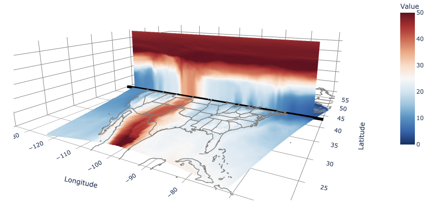
Perspective view of cross-sections
import plotly.graph_objects as go


#plotting parameters
cmap_name='rdbu_r'
geography_color='gray'
cmin,cmax=0,50
# coordinate parameters
i_lev=0
Create geography figures
# Load shapefiles or use built-in geopandas datasets
states = gp.read_file("~/.local/share/cartopy/shapefiles/natural_earth/cultural/ne_50m_admin_1_states_provinces_lakes.shp")
coasts = gp.read_file("~/.local/share/cartopy/shapefiles/natural_earth/physical/ne_50m_coastline.shp")

def extract_polygon_boundaries(gdf):
    boundaries = []
    for geom in gdf.geometry:
        if geom.geom_type == 'Polygon':
            boundaries.append(geom.exterior)
        elif geom.geom_type == 'MultiPolygon':
            for poly in geom.geoms: boundaries.append(poly.exterior)
    return boundaries


def extract_linestring_boundaries(gdf):
    lines = []
    for geom in gdf.geometry:
        if geom.geom_type == 'MultiLineString':
            for line in geom.geoms:lines.append(line)
        elif geom.geom_type == 'LineString':
            lines.append(geom)
    return lines

def make_3d_trace(line,i_lev,min_lat,max_lat,min_lon,max_lon,color='white', width=3):
    lons, lats= line.xy
    lons,lats=np.array(lons),np.array(lats)
    lon_final=lons#[(lons>=min_lon)&(lons<=max_lon)&(lats>=min_lat)&(lons<=max_lat)]
    lat_final=lats#[(lons>=min_lon)&(lons<=max_lon)&(lats>=min_lat)&(lons<=max_lat)]
    lev_final=[i_lev]*lon_final.size
    return go.Scatter3d(x=lon_final, y=lat_final, z=lev_final,mode='lines',line=dict(color=color, width=width),showlegend=False )

boundary_traces = [make_3d_trace(line, i_lev+2,min_lat,max_lat,min_lon,max_lon,color=geography_color) for line in extract_polygon_boundaries(states)]
boundary_traces = [trace for trace in boundary_traces if not (len(trace['x']) == 0 and len(trace['y']) == 0)]

coast_traces = [make_3d_trace(line, i_lev+2,min_lat,max_lat,min_lon,max_lon,color=geography_color) for line in extract_linestring_boundaries(coasts)]
coast_traces = [trace for trace in coast_traces if not (len(trace['x']) == 0 and len(trace['y']) == 0)]
Create horizontal figures and crossections
uxvar_lev0=uxvar.isel(nVertLevels=i_lev)
x = uxvar_lev0.uxgrid.face_lon.values  # longitudes
y = uxvar_lev0.uxgrid.face_lat.values  # latitudes
z = i_lev+np.zeros_like(x)                 # project onto z=0
values = uxvar_lev0.values.transpose()           # scalar field

horizontal_figure=go.Scatter3d(
    name=f'At Level {i_lev:d}',
    x=x,y=y,z=z,
    mode='markers',marker=dict(size=3,color=values,colorscale=cmap_name,cmin=cmin,cmax=cmax)
)


# cross-section along a constant longtiude

# coordinate parameters
lon=-83.3
step_between_points = 400
long_line_x = [lon, lon]
long_line_y = [min_lat, max_lat]
long_line_z = [i_lev, i_lev]

cross_section_lon = uxvar.cross_section(lon=lon, steps=step_between_points)

Long_Line=go.Scatter3d(
    x=long_line_x, y=long_line_y,z=long_line_z,
    mode='lines',line=dict(color='black', width=12),name='Longitude Line'
)

# Create labeled coordinates for plotting
cross_section_lon = cross_section_lon.assign_coords({
    'steps': cross_section_lon['lat'].values,
    'nVertLevels': range(cross_section_lon['nVertLevels'].shape[0])
})

# Get coordinate arrays and create meshgrid
LAT, LEV = np.meshgrid(cross_section_lon['steps'].values, cross_section_lon['nVertLevels'].values, indexing='ij')
LON = lon + np.zeros_like(LAT)

# Flatten for Scatter3d
x,y,z= LON.flatten(), LAT.flatten(), LEV.flatten()  # flip vertical axis if needed
values = cross_section_lon.values.flatten()

# Mask out NaNs
mask = ~np.isnan(values)
x,y,z,values = x[mask],y[mask], z[mask],values[mask]
const_lon_figure=go.Scatter3d(
    name= f"Along {lon:.1f}°{'E' if lon >= 0 else 'W'}",
    x=x,y=y,z=z,mode='markers',opacity=0.8,marker=dict(size=4,color=values,colorscale=cmap_name,cmin=cmin,cmax=cmax)
)

# cross-section along a constant latitude


# coordinate parameters

lat=43.3
step_between_points = 400
lat_line_x = [min_lon, max_lon]
lat_line_y = [lat-0.5, lat-0.5] # slightly deviate the coordinates to show the line out of the background
lat_line_z = [i_lev+1, i_lev+1] # slightly deviate the coordinates to show the line out of the background

Lati_Line=go.Scatter3d(
    x=lat_line_x,y=lat_line_y,z=lat_line_z,
    mode='lines',line=dict(color='black', width=12),name='Latitude Line'
)

cross_section_lat = uxvar.cross_section(lat=lat, steps=step_between_points)

# Create labeled coordinates for plotting
cross_section_lat = cross_section_lat.assign_coords({
    'steps': cross_section_lat['lon'].values,
    'nVertLevels': range(cross_section_lat['nVertLevels'].shape[0])
})

# Get coordinate arrays and create meshgrid
LON, LEV = np.meshgrid(cross_section_lat['steps'].values, cross_section_lat['nVertLevels'].values, indexing='ij')
LAT = lat + np.zeros_like(LON)

# Flatten for Scatter3d
x,y,z= LON.flatten(), LAT.flatten(), LEV.flatten()
values = cross_section_lat.values.flatten()

# Mask out NaNs
mask = ~np.isnan(values)
x,y,z,values = x[mask],y[mask], z[mask],values[mask]

const_lat_figure=go.Scatter3d(
    name= f"Along {lat:.1f}°{'N' if lat >= 0 else 'S'}",
    x=x,y=y,z=z,mode='markers',marker=dict(size=4,color=values,colorscale=cmap_name,cmin=cmin,cmax=cmax,colorbar=dict(title='Value',len=0.6))
)
Updated the figure
Use go.Mesh3d to create a smoother cross-section. It will take a bit more time to render.
# coordinate parameters

lat=43.3
step_between_points = 400
lat_line_x = [min_lon, max_lon]
lat_line_y = [lat-0.5, lat-0.5] # slightly deviate the coordinates to show the line out of the background
lat_line_z = [i_lev+1, i_lev+1] # slightly deviate the coordinates to show the line out of the background

Lati_Line=go.Scatter3d(
    x=lat_line_x,y=lat_line_y,z=lat_line_z,
    mode='lines',line=dict(color='black', width=12),name='Latitude Line'
)

cross_section_lat = uxvar.cross_section(lat=lat, steps=step_between_points)


cross_section_lat = uxvar.cross_section(lat=lat, steps=step_between_points)

# Create labeled coordinates for plotting
cross_section_lat = cross_section_lat.assign_coords({
    'steps': cross_section_lat['lon'].values,
    'nVertLevels': range(cross_section_lat['nVertLevels'].shape[0])
})

# Get coordinate arrays and create meshgrid
LON, LEV = np.meshgrid(cross_section_lat['steps'].values, cross_section_lat['nVertLevels'].values, indexing='ij')
LAT = lat + np.zeros_like(LON)

# Flatten for Scatter3d
x,y,z= LON.flatten(), LAT.flatten(), LEV.flatten()
values = cross_section_lat.values.flatten()

# Build triangle indices before masking
nstep, nlev = len(cross_section_lat['steps']), len(cross_section_lat['nVertLevels'])
i, j, k = [], [], []
for s in range(nstep - 1):
    for l in range(nlev - 1):
        idx = s * nlev + l
        quad = [idx, idx + 1, idx + nlev, idx + nlev + 1]
        if not np.any(np.isnan(values[quad])):
            i += [quad[0], quad[1]]
            j += [quad[1], quad[3]]
            k += [quad[2], quad[2]]

# Mask points and remap indices
valid = ~np.isnan(values)
x, y, z, values = x[valid], y[valid], z[valid], values[valid]
remap = {old: new for new, old in enumerate(np.where(valid)[0])}
i, j, k = [remap[idx] for idx in i], [remap[idx] for idx in j], [remap[idx] for idx in k]

# Add to figure
const_lat_figure = go.Mesh3d(
    name=f"Along {lat:.1f}°{'N' if lat >= 0 else 'S'}",
    x=x, y=y, z=z,i=i, j=j, k=k,intensity=values,
    colorscale=cmap_name,cmin=cmin, cmax=cmax, colorbar=dict(title='Value', len=0.6),showlegend=True,#showscale=True,
    lighting=dict(ambient=1.0),lightposition=dict(x=100, y=200, z=LEV.max()),
    flatshading=True, opacity=1.0,
)
Select and plot figures
fig = go.Figure()
fig.add_trace(horizontal_figure)

for trace in boundary_traces:fig.add_trace(trace)
for trace in coast_traces:fig.add_trace(trace)

# fig.add_trace(const_lon_figure)
# fig.add_trace(Long_Line)

fig.add_trace(const_lat_figure)
fig.add_trace(Lati_Line)

xmin,xmax=min_lon-1, max_lon+1
ymin,ymax=min_lat-1, max_lat+5

fig.update_layout(
    title='UXarray Cross Sections',
    scene=dict(
        xaxis_title='Longitude',yaxis_title='Latitude',zaxis_title='Vertical Level',
        zaxis=dict(range=[LEV.min(),LEV.max()],backgroundcolor="rgba(0,0,0,0)",  gridcolor="gray",    # Grid color for visibility
                    showbackground=True,zerolinecolor="gray"),
        xaxis=dict(range=[xmin,xmax],backgroundcolor="rgba(0,0,0,0)",  gridcolor="gray",
                    showbackground=True,zerolinecolor="gray"),
        yaxis=dict(range=[ymin,ymax],backgroundcolor="rgba(0,0,0,0)",  gridcolor="gray",
                    showbackground=True,zerolinecolor="gray"),
        camera=dict(eye=dict(x=-1.5, y=-3, z=0.4)),
        aspectmode='manual',
        aspectratio=dict(x=1., y=2*(ymax-ymin)/(xmax-xmin), z=0.3),  # Compress z-axis

        bgcolor="rgba(0,0,0,0)" # Transparent background for the entire scene

    ),
    width=1000, height=700
)

fig.show()
Zonal Average
In this session we use the first level and extract its zonal averages at each latitude, with a bin width of 1°:
uxvar_slice=uxvar.isel(nVertLevels=0)

zonal_mean_uxvar=uxvar_slice.zonal_mean((int(min_lat)+1,int(max_lat), 1))
(
    hv.operation.contours(
        uxvar_slice.plot(),
        filled=True,
        ).opts(
        xlim=(int(min_lon-5),int(max_lon)+5),ylim=(int(min_lat-5),int(max_lat)+5),
        cmap="inferno",line_color=None,
        height=250, width=500,
        colorbar=True,colorbar_position='left'
            )* coast_lines * state_lines

    + zonal_mean_uxvar.hvplot.line(
        x="theta_zonal_mean",y="latitudes",
        height=250,width=150,
        ylabel="",
        ylim=(int(min_lat-5),int(max_lat)+5),
        grid=True,
        )

).opts(
    title="Combined Raster and Zonal Average Plot",
    shared_axes=True,
      )
zonal_mean uses a face-weighted average. It accounts for the area of each grid cell, ensuring that larger cells contribute proportionally more to the mean. This is crucial for MPAS grids, which are unstructured and vary in size.
Decompose into zonal averages and zonal anomalies
The total field at any grid could be decomposed into the zonal average, , and the deviations from the zonal average , where represent the latitudinal and longitudinal coordinates, correspondinly.
Why this matters?
The eddy components, or the zonal asymmetrical components, often capture localized variations beyond the zonal mean state. This decomposition is useful when analyzing atmospheric circulation patterns.
# Get latitudes for each face

face_lats = uxvar_slice.uxgrid.face_lat.values  # shape: (n_face,)

#display(zonal_mean_uxvar)

lat_bins = zonal_mean_uxvar['latitudes']
lat_bin_indices = np.digitize(face_lats, lat_bins) - 1

# Clip to valid range
lat_bin_indices = np.clip(lat_bin_indices, 0, len(lat_bins) - 1)

# Map zonal mean to each face
zonal_mean_per_face = zonal_mean_uxvar.values[lat_bin_indices]

# Subtract to get anomaly
uxvar_anomaly = uxvar_slice - zonal_mean_per_face
(
    hv.operation.contours(
        uxvar_anomaly.plot(),
        filled=True,
        ).opts(
        xlim=(int(min_lon-5),int(max_lon)+5),ylim=(int(min_lat-5),int(max_lat)+5),
        cmap="coolwarm",line_color=None,
        height=250, width=500,
        colorbar=True,colorbar_position='left'
            )* coast_lines * state_lines

    + zonal_mean_uxvar.hvplot.line(
        x="theta_zonal_mean",
        y="latitudes",

        height=250,
        width=150,
        ylabel="",
        ylim=(int(min_lat-5),int(max_lat)+5),
        grid=True,
    )
).opts(
    title="Combined Zonal Anomaly & Zonal Average Plot",
      )