Customization & Interactivity
In this tutorial, you’ll learn about:
Switching between Bokeh and Matplotlib backends for different rendering capabilities
Setting up default plot parameters to maintain consistent styling across visualizations
Using dynamic rasterization
Leveraging Bokeh’s interactive features for data exploration, including zooming, panning, and hover tools
Introduction
An essential feature of UXarray is its seamless integration with hvPlot, a powerful plotting library that provides extensive customization and interactivity capabilities. This integration means that when you create visualizations using UXarray, you have access to most of hvPlot’s features for tailoring your plots and making them interactive.
import cartopy.crs as ccrs
import holoviews as hv
import uxarray as ux
from IPython.display import Image
grid_path = "../../meshfiles/oQU480.grid.nc"
data_path = "../../meshfiles/oQU480.data.nc"

uxds = ux.open_dataset(grid_path, data_path)
Plot Parameters
For a comprehensive understanding of the available customization options, please refer to the hvPlot Customization Guide.
Rather than duplicating the extensive documentation available in hvPlot’s user guide, we encourage you to familiarize yourself with their customization options directly. This will provide you with the complete range of parameters available for tailoring your visualizations to meet your specific requirements.
Selecting a Renderer
One key advantage is the flexibility to choose your preferred plotting backend. While Bokeh serves as the default renderer, you can easily switch to Matplotlib by specifying the backend parameter in your plotting commands. This allows you to leverage the unique strengths of each renderer – Bokeh’s interactive features or Matplotlib’s publication-quality static plots.
hv.extension("bokeh")
uxds["bottomDepth"].plot()

# can also do the following
# uxds["bottomDepth"].plot(backend='bokeh')
hv.extension("matplotlib")
uxds["bottomDepth"].plot()

# can also do the following
# uxds["bottomDepth"].plot(backend='matplotlib')
Setting Default Parameters
When creating multiple visualizations, you may want to maintain consistent styling across your plots. HoloViews provides a convenient way to set default parameters through hv.opts.defaults, eliminating the need to repeatedly specify the same parameters for each plot.
In the example below,we set default parameters for all Polygon plots using hv.opts.defaults(hv.opts.Polygons()). The specified parameters: width of 600 pixels, height of 300 pixels, and a default title, will automatically apply to any subsequent Polygon plots unless explicitly overridden.
This approach is particularly useful when developing consistent visualizations for reports or presentations. Rather than manually setting dimensions and styling for each plot, you can establish these parameters once at the beginning of your notebook. This not only saves time but also ensures visual consistency throughout your analysis.
Default parameters can be updated at any point in your notebook, giving you the flexibility to modify the styling of subsequent plots while maintaining the efficiency of centralized parameter management.
hv.extension("bokeh")
hv.opts.defaults(hv.opts.Polygons(width=600, title="My Default Title", height=300))
uxds["bottomDepth"].plot()
Dynamic Rendering
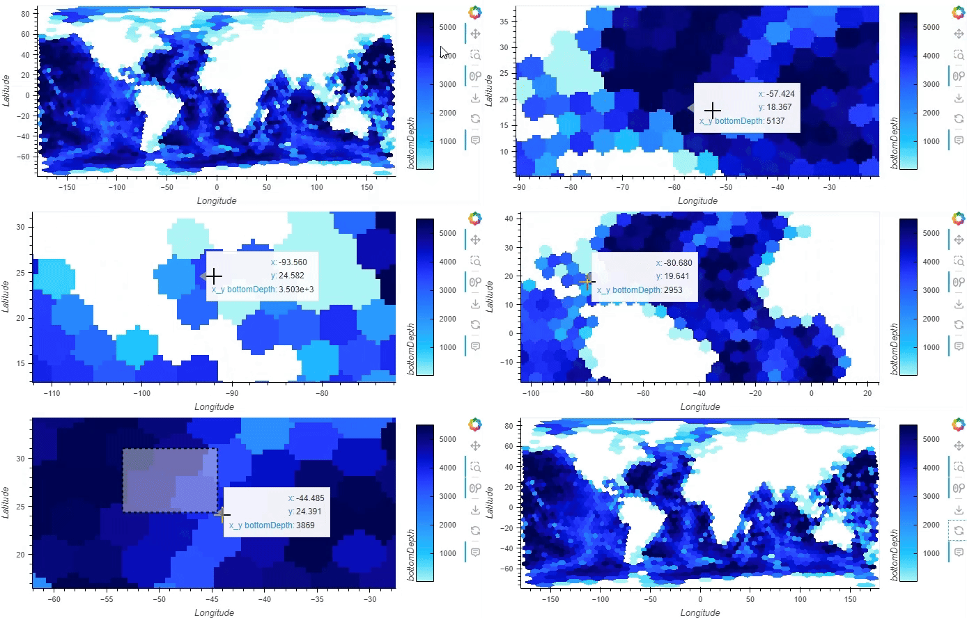
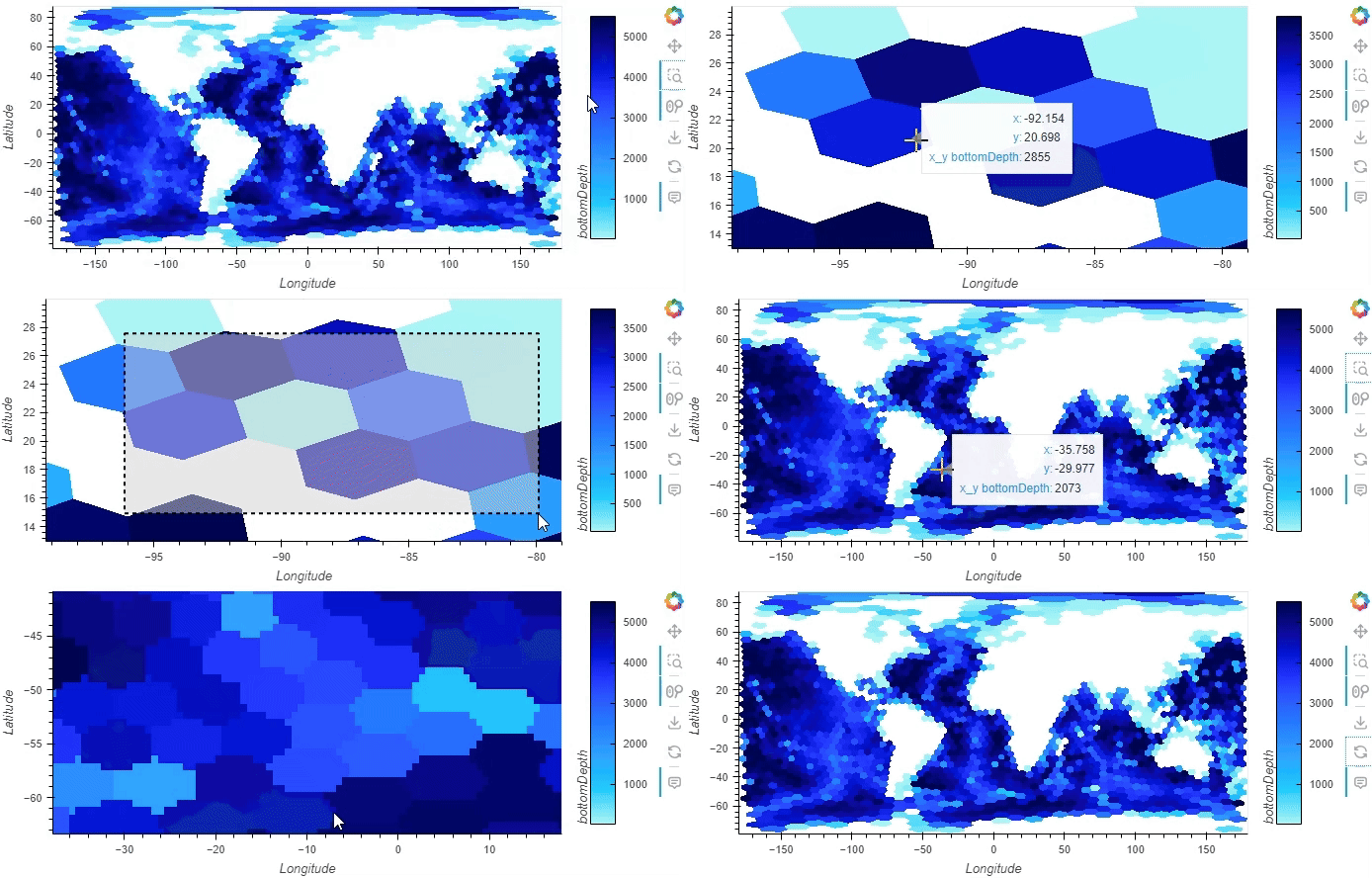
UXarray leverages hvPlot’s dynamic rasterization feature through the dynamic=True parameter. This capability automatically adjusts the plot’s resolution based on your current view, ensuring optimal performance without sacrificing data fidelity.
As you zoom into specific regions of your plot, the visualization engine recalculates and re-rasterizes the data for your current viewport. This means you’ll see increasing levels of detail as you examine smaller areas, revealing fine structures that might not be visible in the full-scale view. This adaptive approach maintains interactive performance while providing high-resolution details where they matter most.
For example, when examining a global ocean mesh, you might start with a view of the entire grid. Upon zooming into a coastal region, the dynamic rasterization automatically refines the visualization, showing intricate mesh elements and local features that were previously aggregated in the broader view. This functionality is particularly valuable when working with multi-resolution meshes or datasets with varying spatial density.
Since the rendered notebooks do not perform the re-rasterization, two GIFs have been provided with commented out code blocks. If you are working on this notebook locally, you can uncomment the code and explore the behavior interactively.
hv.extension("bokeh")
# uxds['bottomDepth'].plot()

# uxds['bottomDepth'].plot(dynamic=True)


