![]()
Py-Art, Xradar y Wradlib
Introducción
En este cuadernillo (Notebook) aprenderemos los conceptos básicos para trabajar con datos provenientes de radares meteorológicos:
Breve introducción a Py-Art
Breve introducción a Xradar
Breve introducción a Wradlib
Prerequisitos
Conceptos |
Importancia |
Notas |
|---|---|---|
Necesario |
Información complementaria |
|
Necesario |
Información complementaria |
|
Necesario |
Generación de gráficas |
|
Necesario |
Generación de mapas |
|
Necesario |
Información complementaria |
Tiempo de aprendizaje: 30 minutos
Librerías
import cartopy.crs as ccrs
import cmweather
import matplotlib.pyplot as plt
import numpy as np
import pyart
import wradlib as wrl
import xradar as xd
0.3.0

## You are using the Python ARM Radar Toolkit (Py-ART), an open source
## library for working with weather radar data. Py-ART is partly
## supported by the U.S. Department of Energy as part of the Atmospheric
## Radiation Measurement (ARM) Climate Research Facility, an Office of
## Science user facility.
##
## If you use this software to prepare a publication, please cite:
##
##     JJ Helmus and SM Collis, JORS 2016, doi: 10.5334/jors.119
1. Py-Art
Py-ARTes una librería en Python que nos permite graficar, corregir y analizar datos de radares meteorológicos de diferentes fabricantes, tipo, y modos de operación. El software ha sido lanzado enGitHubcomo software de código abierto bajo una licencia BSD. Se ejecuta enLinux,OSyWindows.
1.1 Lectura de datos usando Py-Art
Para leer nuestros datos de radar -en el caso particular de este taller usaremos datos provenientes de radares meteorológicos con formato SIGMET- podemos usar el módulo pyart.io.read_sigmet. Sin embargo, Py-Art tiene un módulo I/O mucho más amplio donde se pueden leer datos de otras fuentes o tipos de radares.
radar_pa = pyart.io.read_sigmet(f"../data/CAR220809191504.RAWDSX2")
/usr/share/miniconda3/envs/atmoscol2023/lib/python3.11/site-packages/pyart/io/sigmet.py:146: RuntimeWarning: invalid value encountered in sqrt
  sigmet_data, sigmet_metadata = sigmetfile.read_data(full_xhdr=full_xhdr)
Ahora podemos consultar la información contenida dentro del objeto radar usando rada.info('compact')
radar_pa.info("compact")
altitude: <ndarray of type: float64 and shape: (1,)>
altitude_agl: None
antenna_transition: None
azimuth: <ndarray of type: float32 and shape: (720,)>
elevation: <ndarray of type: float32 and shape: (720,)>
fields:
	total_power: <ndarray of type: float32 and shape: (720, 994)>
	reflectivity: <ndarray of type: float32 and shape: (720, 994)>
	velocity: <ndarray of type: float32 and shape: (720, 994)>
	spectrum_width: <ndarray of type: float32 and shape: (720, 994)>
	differential_reflectivity: <ndarray of type: float32 and shape: (720, 994)>
	specific_differential_phase: <ndarray of type: float32 and shape: (720, 994)>
	differential_phase: <ndarray of type: float32 and shape: (720, 994)>
	normalized_coherent_power: <ndarray of type: float32 and shape: (720, 994)>
	cross_correlation_ratio: <ndarray of type: float32 and shape: (720, 994)>
	radar_echo_classification: <ndarray of type: float32 and shape: (720, 994)>
fixed_angle: <ndarray of type: float32 and shape: (1,)>
instrument_parameters:
	unambiguous_range: <ndarray of type: float32 and shape: (720,)>
	prt_mode: <ndarray of type: |S4 and shape: (1,)>
	prt: <ndarray of type: float32 and shape: (720,)>
	prt_ratio: <ndarray of type: float32 and shape: (720,)>
	nyquist_velocity: <ndarray of type: float32 and shape: (720,)>
	radar_beam_width_h: <ndarray of type: float32 and shape: (1,)>
	radar_beam_width_v: <ndarray of type: float32 and shape: (1,)>
	pulse_width: <ndarray of type: float32 and shape: (720,)>
	prf_flag: <ndarray of type: int16 and shape: (720,)>
latitude: <ndarray of type: float64 and shape: (1,)>
longitude: <ndarray of type: float64 and shape: (1,)>
nsweeps: 1
ngates: 994
nrays: 720
radar_calibration: None
range: <ndarray of type: float32 and shape: (994,)>
scan_rate: None
scan_type: ppi
sweep_end_ray_index: <ndarray of type: int32 and shape: (1,)>
sweep_mode: <ndarray of type: |S20 and shape: (1,)>
sweep_number: <ndarray of type: int32 and shape: (1,)>
sweep_start_ray_index: <ndarray of type: int32 and shape: (1,)>
target_scan_rate: None
time: <ndarray of type: float64 and shape: (720,)>
metadata:
	Conventions: CF/Radial instrument_parameters
	version: 1.3
	title:
	institution:
	references:
	source:
	history:
	comment:
	instrument_name: b'carimagua-radar'
	original_container: sigmet
	sigmet_task_name: b'SURVP       '
	sigmet_extended_header: false
	time_ordered: none
	rays_missing: 0
Podemos listar las variables polarimétricas contenidas en este archivo usando radar.fields
list(radar_pa.fields)
['total_power',
 'reflectivity',
 'velocity',
 'spectrum_width',
 'differential_reflectivity',
 'specific_differential_phase',
 'differential_phase',
 'normalized_coherent_power',
 'cross_correlation_ratio',
 'radar_echo_classification']
La variable polarimétrica más popular en es el factor de reflectividad (Z) que es una medida indirecta de la intensidad y el tamaño de las gotas de lluvia. Podemos ver mas información en el objeto radar usando la notación de diccionarios en Python
radar_pa.fields["reflectivity"]
{'units': 'dBZ',
 'standard_name': 'equivalent_reflectivity_factor',
 'long_name': 'Reflectivity',
 'coordinates': 'elevation azimuth range',
 'data': masked_array(
   data=[[18.5, 20.5, 22.5, ..., --, --, --],
         [26.0, 28.0, 29.0, ..., --, --, --],
         [24.0, 25.5, 26.5, ..., --, --, --],
         ...,
         [25.0, 28.0, 30.0, ..., --, --, --],
         [27.5, 30.0, 31.5, ..., --, --, --],
         [26.0, 27.5, 28.5, ..., --, --, --]],
   mask=[[False, False, False, ...,  True,  True,  True],
         [False, False, False, ...,  True,  True,  True],
         [False, False, False, ...,  True,  True,  True],
         ...,
         [False, False, False, ...,  True,  True,  True],
         [False, False, False, ...,  True,  True,  True],
         [False, False, False, ...,  True,  True,  True]],
   fill_value=1e+20,
   dtype=float32),
 '_FillValue': -9999.0}
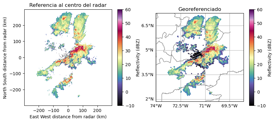
1.2 Gráficas de reflectividad (\(Z\))
Ahora podemos generar salidas gráficas usando el módulo pyart.graph. Esta librería nos permite realizar gráficos con o sin georeferenciacion usando pyart.graph.RadarDisplay o pyart.graph.RadarMapDisplay
fig = plt.figure(figsize=(10, 4))
ax = fig.add_subplot(121)
display_ = pyart.graph.RadarDisplay(radar_pa)
display_.plot(
    "reflectivity",
    0,
    ax=ax,
    colorbar_label="Reflectivity (dBZ)",
    cmap="ChaseSpectral",
    vmin=-10,
    vmax=60,
    title="Referencia al centro del radar",
)

projection = ccrs.PlateCarree()
ax1 = plt.subplot(122, projection=projection)
display_ = pyart.graph.RadarMapDisplay(radar_pa)
# Extraer la latitud y longitud del radar y usarla para centrar el mapa
lat_center = round(radar_pa.latitude["data"][0], 0)
lon_center = round(radar_pa.longitude["data"][0], 0)


# Determinar los anchos
lat_ticks = np.arange(lat_center - 3, lat_center + 3, 1.5)
lon_ticks = np.arange(lon_center - 3, lon_center + 3, 1.5)

# Fijar la proyección - en este caso, usamos la proyección general PlateCarree

display_.plot_ppi_map(
    "reflectivity",
    0,
    resolution="10m",
    ax=ax1,
    lat_lines=lat_ticks,
    lon_lines=lon_ticks,
    colorbar_label="Reflectivity (dBZ)",
    cmap="ChaseSpectral",
    vmin=-10,
    vmax=60,
    title="Georeferenciado",
)
/usr/share/miniconda3/envs/atmoscol2023/lib/python3.11/site-packages/cartopy/io/__init__.py:241: DownloadWarning: Downloading: https://naturalearth.s3.amazonaws.com/10m_physical/ne_10m_coastline.zip
  warnings.warn(f'Downloading: {url}', DownloadWarning)
/usr/share/miniconda3/envs/atmoscol2023/lib/python3.11/site-packages/cartopy/io/__init__.py:241: DownloadWarning: Downloading: https://naturalearth.s3.amazonaws.com/10m_cultural/ne_10m_admin_1_states_provinces_lines.zip
  warnings.warn(f'Downloading: {url}', DownloadWarning)
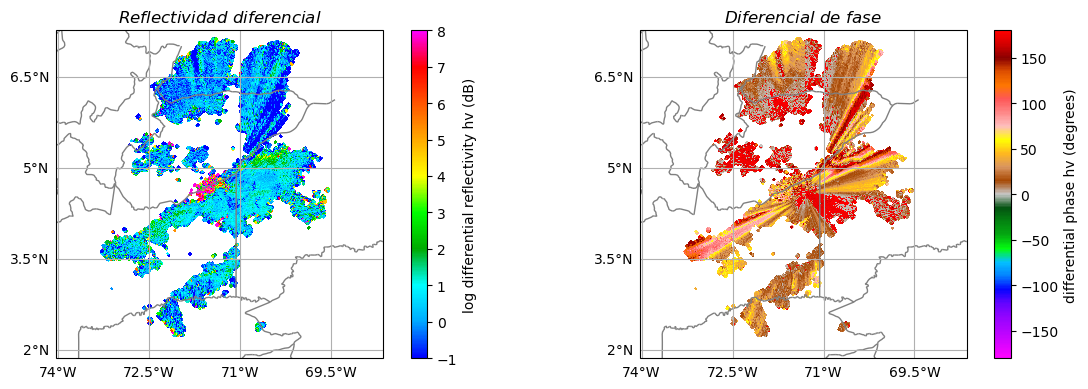
1.3 Gráficas de variables polarimétricas
Tambien podemos generar gráficas de otras variables como reflectividad diferencial (\(Z_{DR}\)), diferencial de fase (\(\phi_{DP}\))
fig = plt.figure(figsize=(12, 4))
display_ = pyart.graph.RadarMapDisplay(radar_pa)

ax2 = plt.subplot(121, projection=projection)
display_.plot_ppi_map(
    "differential_reflectivity",
    0,
    resolution="10m",
    ax=ax2,
    lat_lines=lat_ticks,
    lon_lines=lon_ticks,
    title=r"$Reflectividad \  diferencial$",
)

ax3 = plt.subplot(122, projection=projection)
display_.plot_ppi_map(
    "differential_phase",
    0,
    ax=ax3,
    resolution="10m",
    lat_lines=lat_ticks,
    lon_lines=lon_ticks,
    title=r"$Diferencial \ de \ fase$",
)

plt.tight_layout()
1.4 Otras funcionaldiades de Py-Art
Para más funcionalidades de Py-Art puedes revisar la documentación oficial o el Radar Cookbook donde podras encontrar ejemplos y casos de uso.
2. Xradar
Xradar, de acuerdo con la documentación oficial, “es una herramienta que nos permite incorporar los datos de radar meteorológico al modelo de datos Xarray”. Básicamente, esta herramienta nos permite acceder a nuestros datos de radar usando las ventajas de etiquetas, coordenadas, y atributos. Xradar es una herramienta de código abierto que se basa en la colaboración de la comunidad científica y sus aportes a la misma. Se encuentra en un estado estable y en constante desarrollo.
2.1 Lectura de datos usando Xradar
Al igual que Py-Art, esta librería tiene un módulo I/O que soporta datos de radares de múltiples fuentes/formatos. Para nuestro caso particular, utilizaremos el método xd.io.open_iris_datatree para leer nuestros datos en formato SIGMET.
radar_xd = xd.io.open_iris_datatree(f"../data/CAR220809191504.RAWDSX2")
display(radar_xd)
<xarray.DatasetView>
Dimensions:              ()
Data variables:
    volume_number        int64 0
    platform_type        <U5 'fixed'
    instrument_type      <U5 'radar'
    time_coverage_start  <U20 '2022-08-09T19:15:05Z'
    time_coverage_end    <U20 '2022-08-09T19:16:21Z'
    longitude            float64 -71.33
    altitude             float64 206.0
    latitude             float64 4.564
Attributes:
    Conventions:      None
    version:          None
    title:            None
    institution:      None
    references:       None
    source:           None
    history:          None
    comment:          im/exported using xradar
instrument_name: NoneComo podemos observar nuestro objeto radar tiene una estructura de un xarray.datatree lo que nos permite tener múltiples elevaciones en un solo objeto.
Para acceder a nuestro Dataset podemos usar la notación de diccionarios de Python seguido por el método .ds
display(radar_xd["sweep_0"].ds)
<xarray.DatasetView>
Dimensions:            (azimuth: 720, range: 994)
Coordinates:
    elevation          (azimuth) float32 ...
    time               (azimuth) datetime64[ns] 2022-08-09T19:15:56.891000 .....
  * range              (range) float32 1e+03 1.3e+03 ... 2.986e+05 2.989e+05
    longitude          float64 ...
    latitude           float64 ...
    altitude           float64 ...
  * azimuth            (azimuth) float32 0.03571 0.5795 1.019 ... 359.0 359.6
Data variables: (12/17)
    DBTH               (azimuth, range) float32 ...
    DBZH               (azimuth, range) float32 ...
    VRADH              (azimuth, range) float32 ...
    WRADH              (azimuth, range) float32 ...
    ZDR                (azimuth, range) float32 ...
    KDP                (azimuth, range) float32 ...
    ...                 ...
    DB_DBZE8           (azimuth, range) float32 ...
    sweep_mode         <U20 ...
    sweep_number       int64 ...
    prt_mode           <U7 ...
    follow_mode        <U7 ...
sweep_fixed_angle float64 ...2.2 Gráfico de reflectividad (Z)
Como ya conocemos, Xarray nos permite generar gráficos de manera rápida, sin tener que utilizar la librería matplotlib, usando el método .plot
radar_xd["sweep_0"]["DBZH"].plot(cmap="ChaseSpectral", vmin=-10, vmax=60)
<matplotlib.collections.QuadMesh at 0x7f6136507890>
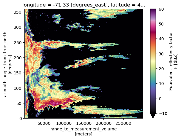
Nuestro Dataset tiene por coordenadas y dimensiones el azimuth y el rango. Debemos georeferenciar nuestro Dataset para visualizar los datos en cordenadas relativas al radar o geográficas. Para lograr esto usamos el método xr.georeference
radar = radar_xd.xradar.georeference()
display(radar["sweep_0"])
<xarray.DatasetView>
Dimensions:            (azimuth: 720, range: 994)
Coordinates:
    elevation          (azimuth) float64 0.4779 0.4779 0.4779 ... 0.4779 0.4779
    time               (azimuth) datetime64[ns] 2022-08-09T19:15:56.891000 .....
  * range              (range) float32 1e+03 1.3e+03 ... 2.986e+05 2.989e+05
    longitude          float64 -71.33
    latitude           float64 4.564
    altitude           float64 206.0
  * azimuth            (azimuth) float32 0.03571 0.5795 1.019 ... 359.0 359.6
    crs_wkt            int64 0
    x                  (azimuth, range) float64 0.6231 0.8101 ... -2.191e+03
    y                  (azimuth, range) float64 999.9 1.3e+03 ... 2.987e+05
    z                  (azimuth, range) float64 214.4 216.9 ... 7.948e+03
Data variables: (12/17)
    DBTH               (azimuth, range) float32 ...
    DBZH               (azimuth, range) float32 ...
    VRADH              (azimuth, range) float32 ...
    WRADH              (azimuth, range) float32 ...
    ZDR                (azimuth, range) float32 ...
    KDP                (azimuth, range) float32 ...
    ...                 ...
    DB_DBZE8           (azimuth, range) float32 ...
    sweep_mode         <U20 ...
    sweep_number       int64 ...
    prt_mode           <U7 ...
    follow_mode        <U7 ...
sweep_fixed_angle float64 ...Como se puede observar, x, y y z han sido agregados como coordenadas a nuestro Dataset.
radar_xd["sweep_0"].x
<xarray.DataArray 'x' (azimuth: 720, range: 994)>
array([[ 6.23142271e-01,  8.10084711e-01,  9.97027039e-01, ...,
         1.85753047e+02,  1.85939651e+02,  1.86126254e+02],
       [ 1.01139065e+01,  1.31480746e+01,  1.61822408e+01, ...,
         3.01486360e+03,  3.01789227e+03,  3.02092094e+03],
       [ 1.77825861e+01,  2.31173550e+01,  2.84521208e+01, ...,
         5.30082727e+03,  5.30615238e+03,  5.31147746e+03],
       ...,
       [-2.48752213e+01, -3.23377781e+01, -3.98003304e+01, ...,
        -7.41507736e+03, -7.42252640e+03, -7.42997541e+03],
       [-1.69676737e+01, -2.20579693e+01, -2.71482618e+01, ...,
        -5.05790930e+03, -5.06299037e+03, -5.06807143e+03],
       [-7.33402886e+00, -9.53423469e+00, -1.17344392e+01, ...,
        -2.18620734e+03, -2.18840356e+03, -2.19059977e+03]])
Coordinates:
elevation (azimuth) float64 0.4779 0.4779 0.4779 ... 0.4779 0.4779 0.4779
time (azimuth) datetime64[ns] 2022-08-09T19:15:56.891000 ... 2022-0...
* range (range) float32 1e+03 1.3e+03 1.6e+03 ... 2.986e+05 2.989e+05
longitude float64 -71.33
latitude float64 4.564
altitude float64 206.0
* azimuth (azimuth) float32 0.03571 0.5795 1.019 ... 358.6 359.0 359.6
crs_wkt int64 0
x (azimuth, range) float64 0.6231 0.8101 ... -2.188e+03 -2.191e+03
y (azimuth, range) float64 999.9 1.3e+03 ... 2.984e+05 2.987e+05
z (azimuth, range) float64 214.4 216.9 ... 7.935e+03 7.948e+03
Attributes:
standard_name: east_west_distance_from_radar
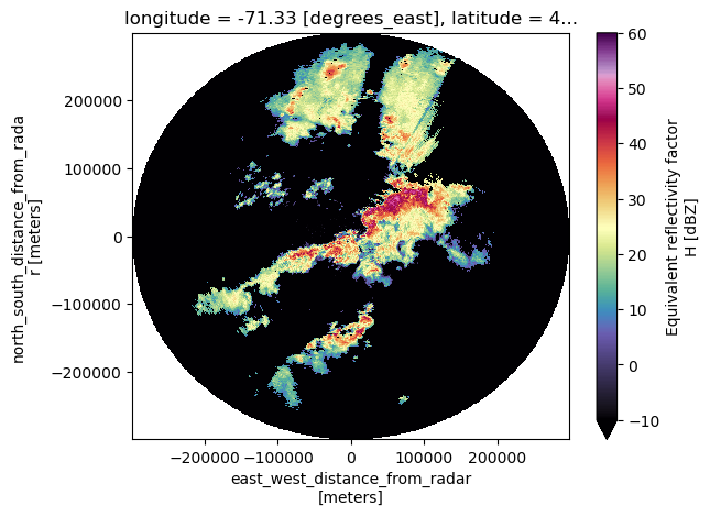
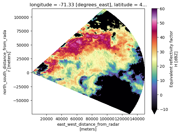
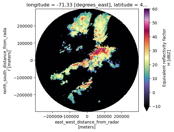
units: metersNuevamente generemos el gráfico de reflectividad pero ahora utilizando las nuevas coordenadas
radar_xd["sweep_0"]["DBZH"].plot(x="x", y="y", cmap="ChaseSpectral", vmin=-10, vmax=60)
<matplotlib.collections.QuadMesh at 0x7f61365e8d90>
2.3 Selección de datos (Slicing)
Como mencionamos en el tutorial de Xarray, podemos utilizar las coordenadas y los atributos para seleccionar datos a lo largo de las dimensiones. Seleccionemos datos de reflecividad entre 40° < azimuth < 120° y 0 < rango < 150km
radar_xd["sweep_0"]["DBZH"].sel(azimuth=slice(40, 120), range=slice(0, 150 * 1e3)).plot(
    x="x", y="y", cmap="ChaseSpectral", vmin=-10, vmax=60
)
<matplotlib.collections.QuadMesh at 0x7f61364a0a90>
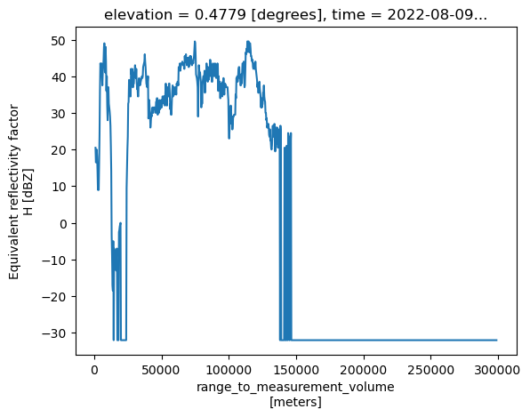
También podemos visualizar la reflectividad en función del rango. Intentémoslo para azimuth=55
radar_xd["sweep_0"]["DBZH"].sel(azimuth=55, method="nearest").plot()
[<matplotlib.lines.Line2D at 0x7f61364a1a90>]
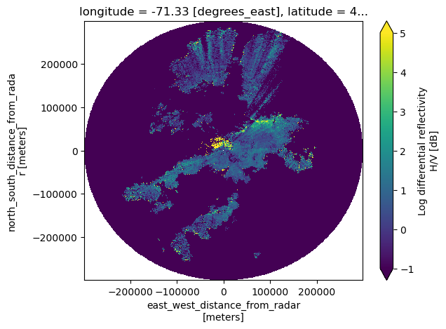
2.4 Acceso a otras variables plorimétricas
Podemos acceder a las variables dentro del Dataset usando la notación de diccionarios de Python o usando el método Punto. Tratemos de acceder a la reflectividad diferencial \(Z_{DR}\)
radar_xd["sweep_0"]["ZDR"].plot(x="x", y="y", vmin=-1, vmax=5)
<matplotlib.collections.QuadMesh at 0x7f61363f0090>
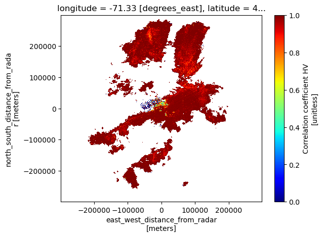
radar_xd["sweep_0"].RHOHV.plot(x="x", y="y", vmin=0, vmax=1, cmap="jet")
/usr/share/miniconda3/envs/atmoscol2023/lib/python3.11/site-packages/xradar/io/backends/iris.py:234: RuntimeWarning: invalid value encountered in sqrt
  return np.sqrt(decode_array(data, **kwargs))
<matplotlib.collections.QuadMesh at 0x7f61362f66d0>
En general, Xradar es una librería relativamente “nueva” que sigue en constante evolución y construcción por parte de la comunidad científica. Para más información pueden consultar la documentación oficial.
3. Wradlib
Wradlib es una librería que, al igual que las anteriores, nos permite acceder a datos de radares meteorológicos de diversas fuentes y formatos. De acuerdo con la documentación oficial “Wradlib está diseñado para ayudar en los pasos más importantes del procesamiento de datos del radar meteorológico. Estos pueden incluir: leer formatos de datos comunes, georreferenciación, convertir la reflectividad en intensidad de lluvia, identificar y corregir fuentes de error típicas (como el desorden o la atenuación) y visualizar los datos”.
3.1 Lectura de datos
Wradlib ofrece un módulo I/O completo para la lectura de archivos de radar en diferentes formatos y plataformas. En nuestro caso, utilizaremos wr.io.read_iris para leer nuestro archivo SIGMET
radar_wrl = wrl.io.read_iris(f"../data/CAR220809191504.RAWDSX2")
radar_wrl.keys()
odict_keys(['product_hdr', 'product_type', 'ingest_header', 'nsweeps', 'nrays', 'nbins', 'data_types', 'data', 'raw_product_bhdrs'])
El objeto retornado es un OrderedDict, que simplemente es un diccionario con unos métodos adicionales a los diccionarios normales de Python. Podemos acceder a las variables polarimétricas del radar de la siguiente manera:
for variable in radar_wrl["data"][1]["ingest_data_hdrs"].keys():
    print(variable)
DB_DBT
DB_DBZ
DB_VEL
DB_WIDTH
DB_ZDR
DB_KDP
DB_PHIDP
DB_SQI
DB_RHOHV
DB_HCLASS
DB_DBTE8
DB_DBZE8
Si queremos acceder a la reflectividad debemos usar la llave DB_DBZ
radar_wrl["data"][1]["sweep_data"]["DB_DBZ"]
array([[ 18.5,  20.5,  22.5, ..., -32. , -32. , -32. ],
       [ 26. ,  28. ,  29. , ..., -32. , -32. , -32. ],
       [ 24. ,  25.5,  26.5, ..., -32. , -32. , -32. ],
       ...,
       [ 25. ,  28. ,  30. , ..., -32. , -32. , -32. ],
       [ 27.5,  30. ,  31.5, ..., -32. , -32. , -32. ],
       [ 26. ,  27.5,  28.5, ..., -32. , -32. , -32. ]])
Puede ser un poco confuso el acceso a los datos usando Wralib. Por lo tanto podemos usar la librería Xradar para acceder a los datos y utilizar los métodos de Wradlib. En el siguiente ejemplo accedemos al sweep_0, luego asignamos coordenadas y georeferencia
swp = radar_xd["sweep_0"].ds.copy()
swp
<xarray.Dataset>
Dimensions:            (azimuth: 720, range: 994)
Coordinates:
    elevation          (azimuth) float64 0.4779 0.4779 0.4779 ... 0.4779 0.4779
    time               (azimuth) datetime64[ns] 2022-08-09T19:15:56.891000 .....
  * range              (range) float32 1e+03 1.3e+03 ... 2.986e+05 2.989e+05
    longitude          float64 -71.33
    latitude           float64 4.564
    altitude           float64 206.0
  * azimuth            (azimuth) float32 0.03571 0.5795 1.019 ... 359.0 359.6
    crs_wkt            int64 0
    x                  (azimuth, range) float64 0.6231 0.8101 ... -2.191e+03
    y                  (azimuth, range) float64 999.9 1.3e+03 ... 2.987e+05
    z                  (azimuth, range) float64 214.4 216.9 ... 7.948e+03
Data variables: (12/17)
    DBTH               (azimuth, range) float32 ...
    DBZH               (azimuth, range) float32 ...
    VRADH              (azimuth, range) float32 ...
    WRADH              (azimuth, range) float32 ...
    ZDR                (azimuth, range) float32 ...
    KDP                (azimuth, range) float32 ...
    ...                 ...
    DB_DBZE8           (azimuth, range) float32 ...
    sweep_mode         <U20 ...
    sweep_number       int64 ...
    prt_mode           <U7 ...
    follow_mode        <U7 ...
sweep_fixed_angle float64 ...swp = swp.assign_coords(sweep_mode=swp.sweep_mode)
swp = swp.wrl.georef.georeference()
swp
<xarray.Dataset>
Dimensions:            (azimuth: 720, range: 994)
Coordinates: (12/15)
    elevation          (azimuth) float64 0.4779 0.4779 0.4779 ... 0.4779 0.4779
    time               (azimuth) datetime64[ns] 2022-08-09T19:15:56.891000 .....
  * range              (range) float32 1e+03 1.3e+03 ... 2.986e+05 2.989e+05
    longitude          float64 -71.33
    latitude           float64 4.564
    altitude           float64 206.0
    ...                 ...
    x                  (azimuth, range) float64 0.6231 0.8101 ... -2.191e+03
    y                  (azimuth, range) float64 999.9 1.3e+03 ... 2.987e+05
    z                  (azimuth, range) float64 214.1 216.6 ... 7.948e+03
    gr                 (azimuth, range) float64 999.9 1.3e+03 ... 2.987e+05
    rays               (azimuth, range) float32 0.03571 0.03571 ... 359.6 359.6
    bins               (azimuth, range) float32 1e+03 1.3e+03 ... 2.989e+05
Data variables: (12/16)
    DBTH               (azimuth, range) float32 ...
    DBZH               (azimuth, range) float32 ...
    VRADH              (azimuth, range) float32 ...
    WRADH              (azimuth, range) float32 ...
    ZDR                (azimuth, range) float32 ...
    KDP                (azimuth, range) float32 ...
    ...                 ...
    DB_DBTE8           (azimuth, range) float32 ...
    DB_DBZE8           (azimuth, range) float32 ...
    sweep_number       int64 ...
    prt_mode           <U7 ...
    follow_mode        <U7 ...
sweep_fixed_angle float64 ...3.2 Gráficos usando wrl.vis
Finalmente podemos generar el gráfico de reflectividad (Z) usando el módulo de visualización wrl.vis.plot
fig = plt.figure(figsize=(5, 5))
pm = swp.DBZH.wrl.vis.plot(vmin=-10, vmax=60, cmap="ChaseSpectral")
Podemos agregar georeferenciación a nuestro Dataset usando el método wrl.georef.epsg_to_osr. Para nuestro caso utilizaremos epsg:4326 o también llamado WGS84. Ahora podemos ver que nuestras coordenadas x y y estan en coordenadas geográficas.
epsg = wrl.georef.epsg_to_osr(4326)
swp = swp.wrl.georef.georeference(crs=epsg)
swp
<xarray.Dataset>
Dimensions:            (azimuth: 720, range: 994)
Coordinates: (12/15)
    elevation          (azimuth) float64 0.4779 0.4779 0.4779 ... 0.4779 0.4779
    time               (azimuth) datetime64[ns] 2022-08-09T19:15:56.891000 .....
  * range              (range) float32 1e+03 1.3e+03 ... 2.986e+05 2.989e+05
    longitude          float64 -71.33
    latitude           float64 4.564
    altitude           float64 206.0
    ...                 ...
    x                  (azimuth, range) float64 -71.33 -71.33 ... -71.35 -71.35
    y                  (azimuth, range) float64 4.573 4.575 ... 7.262 7.264
    z                  (azimuth, range) float64 214.1 216.6 ... 7.948e+03
    gr                 (azimuth, range) float64 0.009043 0.01176 ... 2.698 2.701
    rays               (azimuth, range) float32 0.03571 0.03571 ... 359.6 359.6
    bins               (azimuth, range) float32 1e+03 1.3e+03 ... 2.989e+05
Data variables: (12/16)
    DBTH               (azimuth, range) float32 ...
    DBZH               (azimuth, range) float64 26.0 27.5 28.5 ... -32.0 -32.0
    VRADH              (azimuth, range) float32 ...
    WRADH              (azimuth, range) float32 ...
    ZDR                (azimuth, range) float32 ...
    KDP                (azimuth, range) float32 ...
    ...                 ...
    DB_DBTE8           (azimuth, range) float32 ...
    DB_DBZE8           (azimuth, range) float32 ...
    sweep_number       int64 ...
    prt_mode           <U7 ...
    follow_mode        <U7 ...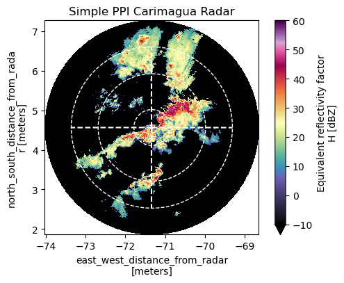
sweep_fixed_angle float64 ...Procedemos ahora a generar un gráfico adicionándole atributos como el centro del radar y unos anillos concéntricos a diferentes distancias usando wrl.vis.plot_ppi_crosshair
fig = plt.figure(figsize=(6, 4))
pm = swp.DBZH.wrl.vis.plot(ax=111, fig=fig, cmap="ChaseSpectral", vmin=-10, vmax=60)
txt = plt.title("Simple PPI Carimagua Radar")

ax = plt.gca()
wrl.vis.plot_ppi_crosshair(
    site=(swp.longitude.values, swp.latitude.values, swp.altitude.values),
    ranges=[50e3, 150e3, 225e3],
    angles=[0, 90, 180, 270],
    line=dict(color="white"),
    circle={"edgecolor": "white"},
    ax=ax,
    crs=epsg,
);
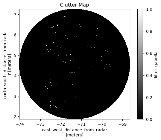
3.3 Mapa de ruido (Clutter)
Entre muchas otras herramientas y funcionalidades, Wradlib nos permite realizar un mapa de ruidos (clutter) usando el filtro desarrollado por Gabella et al. (2002)
clutter = swp.DBZH.wrl.classify.filter_gabella(tr1=12, n_p=6, tr2=1.1)
pm = clutter.wrl.vis.plot(cmap=plt.cm.gray)
plt.title("Clutter Map")
Text(0.5, 1.0, 'Clutter Map')
Wradlib es de librería que nos permite aplicar muchas otras técnicas de filtrado, visualización, estimación cuantitativa de la precipitación, entre otros. Para mas información pueden consultar la documentación oficial.
Conclusiones
En este cuadernillo aprendimos sobre algunas librerías que nos permiten leer y generar productos basados en datos de radares meteorológicos.
Fuentes y referencias
Helmus, J.J. & Collis, S.M., (2016). The Python ARM Radar Toolkit (Py-ART), a Library for Working with Weather Radar Data in the Python Programming Language. Journal of Open Research Software. 4(1), p.e25. DOI: http://doi.org/10.5334/jors.119
Radar Cookbook [https://projectpythia.org/radar-cookbook/README.html] DOI[https://doi.org/10.5281/zenodo.8075855]
Rose, B. E. J., Kent, J., Tyle, K., Clyne, J., Banihirwe, A., Camron, D., May, R., Grover, M., Ford, R. R., Paul, K., Morley, J., Eroglu, O., Kailyn, L., & Zacharias, A. (2023). Pythia Foundations (Version v2023.05.01) https://doi.org/10.5281/zenodo.7884572