
Global Forecast System - GFS
Introducción
En este cuadernillo (Notebook) aprenderemos:
Introducción al GFS
Uso del servidor Thredds
Consulta de datos del GFS a escala de 0.5 grados en resolución usando
siphonVisualización de variables pronosticadas
Prerequisitos
Conceptos |
Importancia |
Notas |
|---|---|---|
Necesario |
Lectura de datos multidimensionales |
|
Necesario |
Entender estampas de tiempo |
|
Útil |
Entender la metadata de los datos |
Tiempo de aprendizaje: 30 minutos
Librerías
Importamos las librerías que vamos a utilizar en este cuadernillo.
from datetime import datetime, timedelta

import cartopy.crs as ccrs
import cartopy.feature as cf
import matplotlib.pyplot as plt
import matplotlib.ticker as mticker
import numpy as np
import xarray as xr
from pandas import to_datetime
from siphon.catalog import TDSCatalog
1. GFS
De acuerdo con la documentación oficial “El Sistema de Pronóstico Global (GFS) es un modelo de pronóstico del tiempo de los Centros Nacionales de Predicción Ambiental (NCEP) que genera datos para docenas de variables atmosféricas y de suelo-suelo, incluidas temperaturas, vientos, precipitaciones, humedad del suelo y concentración de ozono atmosférico.”

Fuente: https://www.ncei.noaa.gov/
Sistema de Pronóstico Global
Utilizado comunmente como condiciones iniciales para otros modelos de pronóstico
El modelo se ejecuta 4 veces al día (00z, 06z, 12z y 18z)
Prósticos de hasta 16 días. 120 primeras horas son a escala horaria, luego cada 3 horas
Modelo tiene 127 capas en la vertical
Utiliza un esquema de esfera cúbica de volumen finito (FV3)
Resolución/dominio horizontal de 0.5, 1.0 y 2.5 grados
2. Acceso a datos del GFS
El acceso a los datos del GFS se puede realizar mediante la descarga directa de los datos utilizando el repositorio de datos del NCEI (National Centers for Environmental Information), usando el repositorio de datos de AWS, o usando el servidor Thredds de la NCAR. Para efectos prácticos del curso, utilizaremos la librería siphon que nos permite realizar consultas al servidor Thredds usando una API en Python.
Para consultar el modelo GFS con resolución espacial de 0.25 grados utilizamos el módulo TDSCatalog y pasamos el link correspondiente que se puede obtener acá.
gfs_url = "http://thredds.ucar.edu/thredds/catalog/grib/NCEP/GFS/Global_0p25deg/catalog.xml?dataset=grib/NCEP/GFS/Global_0p25deg/Best"
best_gfs = TDSCatalog(gfs_url)
best_gfs
Best GFS Quarter Degree Forecast Time Series
Para acceder a este conjunto de datos usando Xarray.Dataset simplemente creamos un acceso remoto de la siguiente manera
ds_gfs = best_gfs.datasets[0].remote_access(use_xarray=True)
print(f"size: {ds_gfs.nbytes / (1024 ** 3)} GB")
display(ds_gfs)
0.3.0
size: 542.7065934985876 GB
<xarray.Dataset>
Dimensions:                                                                     (
                                                                                 time2: 344,
                                                                                 : 2,
                                                                                 time3: 188,
                                                                                 pressure_difference_layer: 1,
                                                                                 depth_below_surface_layer: 4,
                                                                                 ...
                                                                                 height_above_ground: 1,
                                                                                 height_above_ground5: 2,
                                                                                 height_above_ground3: 3,
                                                                                 height_above_ground2: 7,
                                                                                 sigma: 1,
                                                                                 hybrid: 1)
Coordinates: (12/31)
  * lat                                                                         (lat) float32 ...
  * lon                                                                         (lon) float32 ...
  * time                                                                        (time) datetime64[ns] ...
    reftime                                                                     (time) datetime64[ns] ...
  * time1                                                                       (time1) datetime64[ns] ...
    reftime1                                                                    (time1) datetime64[ns] ...
    ...                                                                          ...
  * isobaric1                                                                   (isobaric1) float32 ...
  * height_above_ground4                                                        (height_above_ground4) float32 ...
  * height_above_ground5                                                        (height_above_ground5) float32 ...
  * sigma                                                                       (sigma) float32 ...
  * hybrid                                                                      (hybrid) float32 ...
  * hybrid1                                                                     (hybrid1) float32 ...
Dimensions without coordinates:
Data variables: (12/180)
    LatLon_Projection                                                           int32 ...
    time2_bounds                                                                (time2, ) datetime64[ns] ...
    time3_bounds                                                                (time3, ) datetime64[ns] ...
    pressure_difference_layer_bounds                                            (pressure_difference_layer, ) float32 ...
    depth_below_surface_layer_bounds                                            (depth_below_surface_layer, ) float32 ...
    height_above_ground_layer_bounds                                            (height_above_ground_layer, ) float32 ...
    ...                                                                          ...
    Pressure_potential_vorticity_surface                                        (time, potential_vorticity_surface, lat, lon) float32 ...
    Temperature_potential_vorticity_surface                                     (time, potential_vorticity_surface, lat, lon) float32 ...
    u-component_of_wind_potential_vorticity_surface                             (time, potential_vorticity_surface, lat, lon) float32 ...
    v-component_of_wind_potential_vorticity_surface                             (time, potential_vorticity_surface, lat, lon) float32 ...
    Geopotential_height_potential_vorticity_surface                             (time, potential_vorticity_surface, lat, lon) float32 ...
    Medium_cloud_cover_middle_cloud_Mixed_intervals_Average                     (time3, lat, lon) float32 ...
Attributes:
    Originating_or_generating_Center:                                        ...
    Originating_or_generating_Subcenter:                                     ...
    GRIB_table_version:                                                      ...
    Type_of_generating_process:                                              ...
    Analysis_or_forecast_generating_process_identifier_defined_by_originating...
    file_format:                                                             ...
    Conventions:                                                             ...
    history:                                                                 ...
    featureType:                                                             ...
_CoordSysBuilder: ...- time2: 344
- : 2
- time3: 188
- pressure_difference_layer: 1
- depth_below_surface_layer: 4
- height_above_ground_layer: 1
- height_above_ground_layer1: 1
- pressure_difference_layer1: 1
- pressure_difference_layer2: 3
- sigma_layer: 4
- time: 189
- lat: 721
- lon: 1440
- isobaric: 41
- time1: 188
- potential_vorticity_surface: 2
- isobaric1: 22
- height_above_ground4: 1
- altitude_above_msl: 3
- altitude_above_msl1: 1
- hybrid1: 2
- height_above_ground1: 2
- height_above_ground: 1
- height_above_ground5: 2
- height_above_ground3: 3
- height_above_ground2: 7
- sigma: 1
- hybrid: 1
- lat(lat)float3290.0 89.75 89.5 ... -89.75 -90.0
- units :
- degrees_north
- _CoordinateAxisType :
- Lat
array([ 90. , 89.75, 89.5 , ..., -89.5 , -89.75, -90. ], dtype=float32)
- lon(lon)float320.0 0.25 0.5 ... 359.2 359.5 359.8
- units :
- degrees_east
- _CoordinateAxisType :
- Lon
array([0.0000e+00, 2.5000e-01, 5.0000e-01, ..., 3.5925e+02, 3.5950e+02, 3.5975e+02], dtype=float32) - time(time)datetime64[ns]2023-11-05 ... 2023-11-28T12:00:00
- standard_name :
- time
- long_name :
- GRIB forecast or observation time
- _CoordinateAxisType :
- Time
array(['2023-11-05T00:00:00.000000000', '2023-11-05T03:00:00.000000000', '2023-11-05T06:00:00.000000000', '2023-11-05T09:00:00.000000000', '2023-11-05T12:00:00.000000000', '2023-11-05T15:00:00.000000000', '2023-11-05T18:00:00.000000000', '2023-11-05T21:00:00.000000000', '2023-11-06T00:00:00.000000000', '2023-11-06T03:00:00.000000000', '2023-11-06T06:00:00.000000000', '2023-11-06T09:00:00.000000000', '2023-11-06T12:00:00.000000000', '2023-11-06T15:00:00.000000000', '2023-11-06T18:00:00.000000000', '2023-11-06T21:00:00.000000000', '2023-11-07T00:00:00.000000000', '2023-11-07T03:00:00.000000000', '2023-11-07T06:00:00.000000000', '2023-11-07T09:00:00.000000000', '2023-11-07T12:00:00.000000000', '2023-11-07T15:00:00.000000000', '2023-11-07T18:00:00.000000000', '2023-11-07T21:00:00.000000000', '2023-11-08T00:00:00.000000000', '2023-11-08T03:00:00.000000000', '2023-11-08T06:00:00.000000000', '2023-11-08T09:00:00.000000000', '2023-11-08T12:00:00.000000000', '2023-11-08T15:00:00.000000000', '2023-11-08T18:00:00.000000000', '2023-11-08T21:00:00.000000000', '2023-11-09T00:00:00.000000000', '2023-11-09T03:00:00.000000000', '2023-11-09T06:00:00.000000000', '2023-11-09T09:00:00.000000000', '2023-11-09T12:00:00.000000000', '2023-11-09T15:00:00.000000000', '2023-11-09T18:00:00.000000000', '2023-11-09T21:00:00.000000000', '2023-11-10T00:00:00.000000000', '2023-11-10T03:00:00.000000000', '2023-11-10T06:00:00.000000000', '2023-11-10T09:00:00.000000000', '2023-11-10T12:00:00.000000000', '2023-11-10T15:00:00.000000000', '2023-11-10T18:00:00.000000000', '2023-11-10T21:00:00.000000000', '2023-11-11T00:00:00.000000000', '2023-11-11T03:00:00.000000000', '2023-11-11T06:00:00.000000000', '2023-11-11T09:00:00.000000000', '2023-11-11T12:00:00.000000000', '2023-11-11T15:00:00.000000000', '2023-11-11T18:00:00.000000000', '2023-11-11T21:00:00.000000000', '2023-11-12T00:00:00.000000000', '2023-11-12T03:00:00.000000000', '2023-11-12T06:00:00.000000000', '2023-11-12T09:00:00.000000000', '2023-11-12T12:00:00.000000000', '2023-11-12T15:00:00.000000000', '2023-11-12T18:00:00.000000000', '2023-11-12T21:00:00.000000000', '2023-11-13T00:00:00.000000000', '2023-11-13T03:00:00.000000000', '2023-11-13T06:00:00.000000000', '2023-11-13T09:00:00.000000000', '2023-11-13T12:00:00.000000000', '2023-11-13T15:00:00.000000000', '2023-11-13T18:00:00.000000000', '2023-11-13T21:00:00.000000000', '2023-11-14T00:00:00.000000000', '2023-11-14T03:00:00.000000000', '2023-11-14T06:00:00.000000000', '2023-11-14T09:00:00.000000000', '2023-11-14T12:00:00.000000000', '2023-11-14T15:00:00.000000000', '2023-11-14T18:00:00.000000000', '2023-11-14T21:00:00.000000000', '2023-11-15T00:00:00.000000000', '2023-11-15T03:00:00.000000000', '2023-11-15T06:00:00.000000000', '2023-11-15T09:00:00.000000000', '2023-11-15T12:00:00.000000000', '2023-11-15T15:00:00.000000000', '2023-11-15T18:00:00.000000000', '2023-11-15T21:00:00.000000000', '2023-11-16T00:00:00.000000000', '2023-11-16T03:00:00.000000000', '2023-11-16T06:00:00.000000000', '2023-11-16T09:00:00.000000000', '2023-11-16T12:00:00.000000000', '2023-11-16T15:00:00.000000000', '2023-11-16T18:00:00.000000000', '2023-11-16T21:00:00.000000000', '2023-11-17T00:00:00.000000000', '2023-11-17T03:00:00.000000000', '2023-11-17T06:00:00.000000000', '2023-11-17T09:00:00.000000000', '2023-11-17T12:00:00.000000000', '2023-11-17T15:00:00.000000000', '2023-11-17T18:00:00.000000000', '2023-11-17T21:00:00.000000000', '2023-11-18T00:00:00.000000000', '2023-11-18T03:00:00.000000000', '2023-11-18T06:00:00.000000000', '2023-11-18T09:00:00.000000000', '2023-11-18T12:00:00.000000000', '2023-11-18T15:00:00.000000000', '2023-11-18T18:00:00.000000000', '2023-11-18T21:00:00.000000000', '2023-11-19T00:00:00.000000000', '2023-11-19T03:00:00.000000000', '2023-11-19T06:00:00.000000000', '2023-11-19T09:00:00.000000000', '2023-11-19T12:00:00.000000000', '2023-11-19T15:00:00.000000000', '2023-11-19T18:00:00.000000000', '2023-11-19T21:00:00.000000000', '2023-11-20T00:00:00.000000000', '2023-11-20T03:00:00.000000000', '2023-11-20T06:00:00.000000000', '2023-11-20T09:00:00.000000000', '2023-11-20T12:00:00.000000000', '2023-11-20T15:00:00.000000000', '2023-11-20T18:00:00.000000000', '2023-11-20T21:00:00.000000000', '2023-11-21T00:00:00.000000000', '2023-11-21T03:00:00.000000000', '2023-11-21T06:00:00.000000000', '2023-11-21T09:00:00.000000000', '2023-11-21T12:00:00.000000000', '2023-11-21T15:00:00.000000000', '2023-11-21T18:00:00.000000000', '2023-11-21T21:00:00.000000000', '2023-11-22T00:00:00.000000000', '2023-11-22T03:00:00.000000000', '2023-11-22T06:00:00.000000000', '2023-11-22T09:00:00.000000000', '2023-11-22T12:00:00.000000000', '2023-11-22T15:00:00.000000000', '2023-11-22T18:00:00.000000000', '2023-11-22T21:00:00.000000000', '2023-11-23T00:00:00.000000000', '2023-11-23T03:00:00.000000000', '2023-11-23T06:00:00.000000000', '2023-11-23T09:00:00.000000000', '2023-11-23T12:00:00.000000000', '2023-11-23T15:00:00.000000000', '2023-11-23T18:00:00.000000000', '2023-11-23T21:00:00.000000000', '2023-11-24T00:00:00.000000000', '2023-11-24T03:00:00.000000000', '2023-11-24T06:00:00.000000000', '2023-11-24T09:00:00.000000000', '2023-11-24T12:00:00.000000000', '2023-11-24T15:00:00.000000000', '2023-11-24T18:00:00.000000000', '2023-11-24T21:00:00.000000000', '2023-11-25T00:00:00.000000000', '2023-11-25T03:00:00.000000000', '2023-11-25T06:00:00.000000000', '2023-11-25T09:00:00.000000000', '2023-11-25T12:00:00.000000000', '2023-11-25T15:00:00.000000000', '2023-11-25T18:00:00.000000000', '2023-11-25T21:00:00.000000000', '2023-11-26T00:00:00.000000000', '2023-11-26T03:00:00.000000000', '2023-11-26T06:00:00.000000000', '2023-11-26T09:00:00.000000000', '2023-11-26T12:00:00.000000000', '2023-11-26T15:00:00.000000000', '2023-11-26T18:00:00.000000000', '2023-11-26T21:00:00.000000000', '2023-11-27T00:00:00.000000000', '2023-11-27T03:00:00.000000000', '2023-11-27T06:00:00.000000000', '2023-11-27T09:00:00.000000000', '2023-11-27T12:00:00.000000000', '2023-11-27T15:00:00.000000000', '2023-11-27T18:00:00.000000000', '2023-11-27T21:00:00.000000000', '2023-11-28T00:00:00.000000000', '2023-11-28T03:00:00.000000000', '2023-11-28T06:00:00.000000000', '2023-11-28T09:00:00.000000000', '2023-11-28T12:00:00.000000000'], dtype='datetime64[ns]') - reftime(time)datetime64[ns]...
- standard_name :
- forecast_reference_time
- long_name :
- GRIB reference time
- _CoordinateAxisType :
- RunTime
[189 values with dtype=datetime64[ns]]
- time1(time1)datetime64[ns]2023-11-05T03:00:00 ... 2023-11-...
- standard_name :
- time
- long_name :
- GRIB forecast or observation time
- _CoordinateAxisType :
- Time
array(['2023-11-05T03:00:00.000000000', '2023-11-05T06:00:00.000000000', '2023-11-05T09:00:00.000000000', '2023-11-05T12:00:00.000000000', '2023-11-05T15:00:00.000000000', '2023-11-05T18:00:00.000000000', '2023-11-05T21:00:00.000000000', '2023-11-06T00:00:00.000000000', '2023-11-06T03:00:00.000000000', '2023-11-06T06:00:00.000000000', '2023-11-06T09:00:00.000000000', '2023-11-06T12:00:00.000000000', '2023-11-06T15:00:00.000000000', '2023-11-06T18:00:00.000000000', '2023-11-06T21:00:00.000000000', '2023-11-07T00:00:00.000000000', '2023-11-07T03:00:00.000000000', '2023-11-07T06:00:00.000000000', '2023-11-07T09:00:00.000000000', '2023-11-07T12:00:00.000000000', '2023-11-07T15:00:00.000000000', '2023-11-07T18:00:00.000000000', '2023-11-07T21:00:00.000000000', '2023-11-08T00:00:00.000000000', '2023-11-08T03:00:00.000000000', '2023-11-08T06:00:00.000000000', '2023-11-08T09:00:00.000000000', '2023-11-08T12:00:00.000000000', '2023-11-08T15:00:00.000000000', '2023-11-08T18:00:00.000000000', '2023-11-08T21:00:00.000000000', '2023-11-09T00:00:00.000000000', '2023-11-09T03:00:00.000000000', '2023-11-09T06:00:00.000000000', '2023-11-09T09:00:00.000000000', '2023-11-09T12:00:00.000000000', '2023-11-09T15:00:00.000000000', '2023-11-09T18:00:00.000000000', '2023-11-09T21:00:00.000000000', '2023-11-10T00:00:00.000000000', '2023-11-10T03:00:00.000000000', '2023-11-10T06:00:00.000000000', '2023-11-10T09:00:00.000000000', '2023-11-10T12:00:00.000000000', '2023-11-10T15:00:00.000000000', '2023-11-10T18:00:00.000000000', '2023-11-10T21:00:00.000000000', '2023-11-11T00:00:00.000000000', '2023-11-11T03:00:00.000000000', '2023-11-11T06:00:00.000000000', '2023-11-11T09:00:00.000000000', '2023-11-11T12:00:00.000000000', '2023-11-11T15:00:00.000000000', '2023-11-11T18:00:00.000000000', '2023-11-11T21:00:00.000000000', '2023-11-12T00:00:00.000000000', '2023-11-12T03:00:00.000000000', '2023-11-12T06:00:00.000000000', '2023-11-12T09:00:00.000000000', '2023-11-12T12:00:00.000000000', '2023-11-12T15:00:00.000000000', '2023-11-12T18:00:00.000000000', '2023-11-12T21:00:00.000000000', '2023-11-13T00:00:00.000000000', '2023-11-13T03:00:00.000000000', '2023-11-13T06:00:00.000000000', '2023-11-13T09:00:00.000000000', '2023-11-13T12:00:00.000000000', '2023-11-13T15:00:00.000000000', '2023-11-13T18:00:00.000000000', '2023-11-13T21:00:00.000000000', '2023-11-14T00:00:00.000000000', '2023-11-14T03:00:00.000000000', '2023-11-14T06:00:00.000000000', '2023-11-14T09:00:00.000000000', '2023-11-14T12:00:00.000000000', '2023-11-14T15:00:00.000000000', '2023-11-14T18:00:00.000000000', '2023-11-14T21:00:00.000000000', '2023-11-15T00:00:00.000000000', '2023-11-15T03:00:00.000000000', '2023-11-15T06:00:00.000000000', '2023-11-15T09:00:00.000000000', '2023-11-15T12:00:00.000000000', '2023-11-15T15:00:00.000000000', '2023-11-15T18:00:00.000000000', '2023-11-15T21:00:00.000000000', '2023-11-16T00:00:00.000000000', '2023-11-16T03:00:00.000000000', '2023-11-16T06:00:00.000000000', '2023-11-16T09:00:00.000000000', '2023-11-16T12:00:00.000000000', '2023-11-16T15:00:00.000000000', '2023-11-16T18:00:00.000000000', '2023-11-16T21:00:00.000000000', '2023-11-17T00:00:00.000000000', '2023-11-17T03:00:00.000000000', '2023-11-17T06:00:00.000000000', '2023-11-17T09:00:00.000000000', '2023-11-17T12:00:00.000000000', '2023-11-17T15:00:00.000000000', '2023-11-17T18:00:00.000000000', '2023-11-17T21:00:00.000000000', '2023-11-18T00:00:00.000000000', '2023-11-18T03:00:00.000000000', '2023-11-18T06:00:00.000000000', '2023-11-18T09:00:00.000000000', '2023-11-18T12:00:00.000000000', '2023-11-18T15:00:00.000000000', '2023-11-18T18:00:00.000000000', '2023-11-18T21:00:00.000000000', '2023-11-19T00:00:00.000000000', '2023-11-19T03:00:00.000000000', '2023-11-19T06:00:00.000000000', '2023-11-19T09:00:00.000000000', '2023-11-19T12:00:00.000000000', '2023-11-19T15:00:00.000000000', '2023-11-19T18:00:00.000000000', '2023-11-19T21:00:00.000000000', '2023-11-20T00:00:00.000000000', '2023-11-20T03:00:00.000000000', '2023-11-20T06:00:00.000000000', '2023-11-20T09:00:00.000000000', '2023-11-20T12:00:00.000000000', '2023-11-20T15:00:00.000000000', '2023-11-20T18:00:00.000000000', '2023-11-20T21:00:00.000000000', '2023-11-21T00:00:00.000000000', '2023-11-21T03:00:00.000000000', '2023-11-21T06:00:00.000000000', '2023-11-21T09:00:00.000000000', '2023-11-21T12:00:00.000000000', '2023-11-21T15:00:00.000000000', '2023-11-21T18:00:00.000000000', '2023-11-21T21:00:00.000000000', '2023-11-22T00:00:00.000000000', '2023-11-22T03:00:00.000000000', '2023-11-22T06:00:00.000000000', '2023-11-22T09:00:00.000000000', '2023-11-22T12:00:00.000000000', '2023-11-22T15:00:00.000000000', '2023-11-22T18:00:00.000000000', '2023-11-22T21:00:00.000000000', '2023-11-23T00:00:00.000000000', '2023-11-23T03:00:00.000000000', '2023-11-23T06:00:00.000000000', '2023-11-23T09:00:00.000000000', '2023-11-23T12:00:00.000000000', '2023-11-23T15:00:00.000000000', '2023-11-23T18:00:00.000000000', '2023-11-23T21:00:00.000000000', '2023-11-24T00:00:00.000000000', '2023-11-24T03:00:00.000000000', '2023-11-24T06:00:00.000000000', '2023-11-24T09:00:00.000000000', '2023-11-24T12:00:00.000000000', '2023-11-24T15:00:00.000000000', '2023-11-24T18:00:00.000000000', '2023-11-24T21:00:00.000000000', '2023-11-25T00:00:00.000000000', '2023-11-25T03:00:00.000000000', '2023-11-25T06:00:00.000000000', '2023-11-25T09:00:00.000000000', '2023-11-25T12:00:00.000000000', '2023-11-25T15:00:00.000000000', '2023-11-25T18:00:00.000000000', '2023-11-25T21:00:00.000000000', '2023-11-26T00:00:00.000000000', '2023-11-26T03:00:00.000000000', '2023-11-26T06:00:00.000000000', '2023-11-26T09:00:00.000000000', '2023-11-26T12:00:00.000000000', '2023-11-26T15:00:00.000000000', '2023-11-26T18:00:00.000000000', '2023-11-26T21:00:00.000000000', '2023-11-27T00:00:00.000000000', '2023-11-27T03:00:00.000000000', '2023-11-27T06:00:00.000000000', '2023-11-27T09:00:00.000000000', '2023-11-27T12:00:00.000000000', '2023-11-27T15:00:00.000000000', '2023-11-27T18:00:00.000000000', '2023-11-27T21:00:00.000000000', '2023-11-28T00:00:00.000000000', '2023-11-28T03:00:00.000000000', '2023-11-28T06:00:00.000000000', '2023-11-28T09:00:00.000000000', '2023-11-28T12:00:00.000000000'], dtype='datetime64[ns]') - reftime1(time1)datetime64[ns]...
- standard_name :
- forecast_reference_time
- long_name :
- GRIB reference time
- _CoordinateAxisType :
- RunTime
[188 values with dtype=datetime64[ns]]
- time2(time2)datetime64[ns]2023-11-05T03:00:00 ... 2023-11-...
- standard_name :
- time
- long_name :
- GRIB forecast or observation time
- bounds :
- time2_bounds
- _CoordinateAxisType :
- Time
array(['2023-11-05T03:00:00.000000000', '2023-11-05T06:00:00.000000000', '2023-11-05T09:00:00.000000000', ..., '2023-11-28T09:00:00.000000000', '2023-11-28T12:00:00.000000000', '2023-11-28T12:00:00.000000000'], dtype='datetime64[ns]') - reftime2(time2)datetime64[ns]...
- standard_name :
- forecast_reference_time
- long_name :
- GRIB reference time
- _CoordinateAxisType :
- RunTime
[344 values with dtype=datetime64[ns]]
- time3(time3)datetime64[ns]2023-11-05T03:00:00 ... 2023-11-...
- standard_name :
- time
- long_name :
- GRIB forecast or observation time
- bounds :
- time3_bounds
- _CoordinateAxisType :
- Time
array(['2023-11-05T03:00:00.000000000', '2023-11-05T06:00:00.000000000', '2023-11-05T09:00:00.000000000', '2023-11-05T12:00:00.000000000', '2023-11-05T15:00:00.000000000', '2023-11-05T18:00:00.000000000', '2023-11-05T21:00:00.000000000', '2023-11-06T00:00:00.000000000', '2023-11-06T03:00:00.000000000', '2023-11-06T06:00:00.000000000', '2023-11-06T09:00:00.000000000', '2023-11-06T12:00:00.000000000', '2023-11-06T15:00:00.000000000', '2023-11-06T18:00:00.000000000', '2023-11-06T21:00:00.000000000', '2023-11-07T00:00:00.000000000', '2023-11-07T03:00:00.000000000', '2023-11-07T06:00:00.000000000', '2023-11-07T09:00:00.000000000', '2023-11-07T12:00:00.000000000', '2023-11-07T15:00:00.000000000', '2023-11-07T18:00:00.000000000', '2023-11-07T21:00:00.000000000', '2023-11-08T00:00:00.000000000', '2023-11-08T03:00:00.000000000', '2023-11-08T06:00:00.000000000', '2023-11-08T09:00:00.000000000', '2023-11-08T12:00:00.000000000', '2023-11-08T15:00:00.000000000', '2023-11-08T18:00:00.000000000', '2023-11-08T21:00:00.000000000', '2023-11-09T00:00:00.000000000', '2023-11-09T03:00:00.000000000', '2023-11-09T06:00:00.000000000', '2023-11-09T09:00:00.000000000', '2023-11-09T12:00:00.000000000', '2023-11-09T15:00:00.000000000', '2023-11-09T18:00:00.000000000', '2023-11-09T21:00:00.000000000', '2023-11-10T00:00:00.000000000', '2023-11-10T03:00:00.000000000', '2023-11-10T06:00:00.000000000', '2023-11-10T09:00:00.000000000', '2023-11-10T12:00:00.000000000', '2023-11-10T15:00:00.000000000', '2023-11-10T18:00:00.000000000', '2023-11-10T21:00:00.000000000', '2023-11-11T00:00:00.000000000', '2023-11-11T03:00:00.000000000', '2023-11-11T06:00:00.000000000', '2023-11-11T09:00:00.000000000', '2023-11-11T12:00:00.000000000', '2023-11-11T15:00:00.000000000', '2023-11-11T18:00:00.000000000', '2023-11-11T21:00:00.000000000', '2023-11-12T00:00:00.000000000', '2023-11-12T03:00:00.000000000', '2023-11-12T06:00:00.000000000', '2023-11-12T09:00:00.000000000', '2023-11-12T12:00:00.000000000', '2023-11-12T15:00:00.000000000', '2023-11-12T18:00:00.000000000', '2023-11-12T21:00:00.000000000', '2023-11-13T00:00:00.000000000', '2023-11-13T03:00:00.000000000', '2023-11-13T06:00:00.000000000', '2023-11-13T09:00:00.000000000', '2023-11-13T12:00:00.000000000', '2023-11-13T15:00:00.000000000', '2023-11-13T18:00:00.000000000', '2023-11-13T21:00:00.000000000', '2023-11-14T00:00:00.000000000', '2023-11-14T03:00:00.000000000', '2023-11-14T06:00:00.000000000', '2023-11-14T09:00:00.000000000', '2023-11-14T12:00:00.000000000', '2023-11-14T15:00:00.000000000', '2023-11-14T18:00:00.000000000', '2023-11-14T21:00:00.000000000', '2023-11-15T00:00:00.000000000', '2023-11-15T03:00:00.000000000', '2023-11-15T06:00:00.000000000', '2023-11-15T09:00:00.000000000', '2023-11-15T12:00:00.000000000', '2023-11-15T15:00:00.000000000', '2023-11-15T18:00:00.000000000', '2023-11-15T21:00:00.000000000', '2023-11-16T00:00:00.000000000', '2023-11-16T03:00:00.000000000', '2023-11-16T06:00:00.000000000', '2023-11-16T09:00:00.000000000', '2023-11-16T12:00:00.000000000', '2023-11-16T15:00:00.000000000', '2023-11-16T18:00:00.000000000', '2023-11-16T21:00:00.000000000', '2023-11-17T00:00:00.000000000', '2023-11-17T03:00:00.000000000', '2023-11-17T06:00:00.000000000', '2023-11-17T09:00:00.000000000', '2023-11-17T12:00:00.000000000', '2023-11-17T15:00:00.000000000', '2023-11-17T18:00:00.000000000', '2023-11-17T21:00:00.000000000', '2023-11-18T00:00:00.000000000', '2023-11-18T03:00:00.000000000', '2023-11-18T06:00:00.000000000', '2023-11-18T09:00:00.000000000', '2023-11-18T12:00:00.000000000', '2023-11-18T15:00:00.000000000', '2023-11-18T18:00:00.000000000', '2023-11-18T21:00:00.000000000', '2023-11-19T00:00:00.000000000', '2023-11-19T03:00:00.000000000', '2023-11-19T06:00:00.000000000', '2023-11-19T09:00:00.000000000', '2023-11-19T12:00:00.000000000', '2023-11-19T15:00:00.000000000', '2023-11-19T18:00:00.000000000', '2023-11-19T21:00:00.000000000', '2023-11-20T00:00:00.000000000', '2023-11-20T03:00:00.000000000', '2023-11-20T06:00:00.000000000', '2023-11-20T09:00:00.000000000', '2023-11-20T12:00:00.000000000', '2023-11-20T15:00:00.000000000', '2023-11-20T18:00:00.000000000', '2023-11-20T21:00:00.000000000', '2023-11-21T00:00:00.000000000', '2023-11-21T03:00:00.000000000', '2023-11-21T06:00:00.000000000', '2023-11-21T09:00:00.000000000', '2023-11-21T12:00:00.000000000', '2023-11-21T15:00:00.000000000', '2023-11-21T18:00:00.000000000', '2023-11-21T21:00:00.000000000', '2023-11-22T00:00:00.000000000', '2023-11-22T03:00:00.000000000', '2023-11-22T06:00:00.000000000', '2023-11-22T09:00:00.000000000', '2023-11-22T12:00:00.000000000', '2023-11-22T15:00:00.000000000', '2023-11-22T18:00:00.000000000', '2023-11-22T21:00:00.000000000', '2023-11-23T00:00:00.000000000', '2023-11-23T03:00:00.000000000', '2023-11-23T06:00:00.000000000', '2023-11-23T09:00:00.000000000', '2023-11-23T12:00:00.000000000', '2023-11-23T15:00:00.000000000', '2023-11-23T18:00:00.000000000', '2023-11-23T21:00:00.000000000', '2023-11-24T00:00:00.000000000', '2023-11-24T03:00:00.000000000', '2023-11-24T06:00:00.000000000', '2023-11-24T09:00:00.000000000', '2023-11-24T12:00:00.000000000', '2023-11-24T15:00:00.000000000', '2023-11-24T18:00:00.000000000', '2023-11-24T21:00:00.000000000', '2023-11-25T00:00:00.000000000', '2023-11-25T03:00:00.000000000', '2023-11-25T06:00:00.000000000', '2023-11-25T09:00:00.000000000', '2023-11-25T12:00:00.000000000', '2023-11-25T15:00:00.000000000', '2023-11-25T18:00:00.000000000', '2023-11-25T21:00:00.000000000', '2023-11-26T00:00:00.000000000', '2023-11-26T03:00:00.000000000', '2023-11-26T06:00:00.000000000', '2023-11-26T09:00:00.000000000', '2023-11-26T12:00:00.000000000', '2023-11-26T15:00:00.000000000', '2023-11-26T18:00:00.000000000', '2023-11-26T21:00:00.000000000', '2023-11-27T00:00:00.000000000', '2023-11-27T03:00:00.000000000', '2023-11-27T06:00:00.000000000', '2023-11-27T09:00:00.000000000', '2023-11-27T12:00:00.000000000', '2023-11-27T15:00:00.000000000', '2023-11-27T18:00:00.000000000', '2023-11-27T21:00:00.000000000', '2023-11-28T00:00:00.000000000', '2023-11-28T03:00:00.000000000', '2023-11-28T06:00:00.000000000', '2023-11-28T09:00:00.000000000', '2023-11-28T12:00:00.000000000'], dtype='datetime64[ns]') - reftime3(time3)datetime64[ns]...
- standard_name :
- forecast_reference_time
- long_name :
- GRIB reference time
- _CoordinateAxisType :
- RunTime
[188 values with dtype=datetime64[ns]]
- pressure_difference_layer(pressure_difference_layer)float321.275e+04
- units :
- Pa
- long_name :
- Level at specified pressure difference from ground to level
- positive :
- up
- Grib_level_type :
- 108
- datum :
- ground
- bounds :
- pressure_difference_layer_bounds
- _CoordinateAxisType :
- Pressure
- _CoordinateZisPositive :
- up
array([12750.], dtype=float32)
- height_above_ground(height_above_ground)float3280.0
- units :
- m
- long_name :
- Specified height level above ground
- positive :
- up
- Grib_level_type :
- 103
- datum :
- ground
- _CoordinateAxisType :
- Height
- _CoordinateZisPositive :
- up
array([80.], dtype=float32)
- depth_below_surface_layer(depth_below_surface_layer)float320.05 0.25 0.7 1.5
- units :
- m
- long_name :
- Depth below land surface
- positive :
- down
- Grib_level_type :
- 106
- datum :
- land surface
- bounds :
- depth_below_surface_layer_bounds
- _CoordinateAxisType :
- Height
- _CoordinateZisPositive :
- down
array([0.05, 0.25, 0.7 , 1.5 ], dtype=float32)
- height_above_ground1(height_above_ground1)float321e+03 4e+03
- units :
- m
- long_name :
- Specified height level above ground
- positive :
- up
- Grib_level_type :
- 103
- datum :
- ground
- _CoordinateAxisType :
- Height
- _CoordinateZisPositive :
- up
array([1000., 4000.], dtype=float32)
- altitude_above_msl(altitude_above_msl)float321.829e+03 2.743e+03 3.658e+03
- units :
- m
- long_name :
- Specific altitude above mean sea level
- positive :
- up
- Grib_level_type :
- 102
- datum :
- mean sea level
- _CoordinateAxisType :
- Height
- _CoordinateZisPositive :
- up
array([1829., 2743., 3658.], dtype=float32)
- altitude_above_msl1(altitude_above_msl1)float3210.0
- units :
- m
- long_name :
- Specific altitude above mean sea level
- positive :
- up
- Grib_level_type :
- 102
- datum :
- mean sea level
- _CoordinateAxisType :
- Height
- _CoordinateZisPositive :
- up
array([10.], dtype=float32)
- isobaric(isobaric)float321.0 2.0 4.0 ... 9.75e+04 1e+05
- units :
- Pa
- long_name :
- Isobaric surface
- positive :
- down
- Grib_level_type :
- 100
- _CoordinateAxisType :
- Pressure
- _CoordinateZisPositive :
- down
array([1.00e+00, 2.00e+00, 4.00e+00, 7.00e+00, 1.00e+01, 2.00e+01, 4.00e+01, 7.00e+01, 1.00e+02, 2.00e+02, 3.00e+02, 5.00e+02, 7.00e+02, 1.00e+03, 1.50e+03, 2.00e+03, 3.00e+03, 4.00e+03, 5.00e+03, 7.00e+03, 1.00e+04, 1.50e+04, 2.00e+04, 2.50e+04, 3.00e+04, 3.50e+04, 4.00e+04, 4.50e+04, 5.00e+04, 5.50e+04, 6.00e+04, 6.50e+04, 7.00e+04, 7.50e+04, 8.00e+04, 8.50e+04, 9.00e+04, 9.25e+04, 9.50e+04, 9.75e+04, 1.00e+05], dtype=float32) - height_above_ground_layer(height_above_ground_layer)float321.5e+03
- units :
- m
- long_name :
- Specified height level above ground
- positive :
- up
- Grib_level_type :
- 103
- datum :
- ground
- bounds :
- height_above_ground_layer_bounds
- _CoordinateAxisType :
- Height
- _CoordinateZisPositive :
- up
array([1500.], dtype=float32)
- height_above_ground_layer1(height_above_ground_layer1)float323e+03
- units :
- m
- long_name :
- Specified height level above ground
- positive :
- up
- Grib_level_type :
- 103
- datum :
- ground
- bounds :
- height_above_ground_layer1_bounds
- _CoordinateAxisType :
- Height
- _CoordinateZisPositive :
- up
array([3000.], dtype=float32)
- pressure_difference_layer1(pressure_difference_layer1)float321.5e+03
- units :
- Pa
- long_name :
- Level at specified pressure difference from ground to level
- positive :
- up
- Grib_level_type :
- 108
- datum :
- ground
- bounds :
- pressure_difference_layer1_bounds
- _CoordinateAxisType :
- Pressure
- _CoordinateZisPositive :
- up
array([1500.], dtype=float32)
- pressure_difference_layer2(pressure_difference_layer2)float324.5e+03 9e+03 1.275e+04
- units :
- Pa
- long_name :
- Level at specified pressure difference from ground to level
- positive :
- up
- Grib_level_type :
- 108
- datum :
- ground
- bounds :
- pressure_difference_layer2_bounds
- _CoordinateAxisType :
- Pressure
- _CoordinateZisPositive :
- up
array([ 4500., 9000., 12750.], dtype=float32)
- potential_vorticity_surface(potential_vorticity_surface)float32-2e-06 2e-06
- units :
- K m2 kg-1 s-1
- long_name :
- Potential vorticity surface
- positive :
- up
- Grib_level_type :
- 109
- _CoordinateAxisType :
- GeoZ
- _CoordinateZisPositive :
- up
array([-2.e-06, 2.e-06], dtype=float32)
- height_above_ground2(height_above_ground2)float3210.0 20.0 30.0 40.0 50.0 80.0 100.0
- units :
- m
- long_name :
- Specified height level above ground
- positive :
- up
- Grib_level_type :
- 103
- datum :
- ground
- _CoordinateAxisType :
- Height
- _CoordinateZisPositive :
- up
array([ 10., 20., 30., 40., 50., 80., 100.], dtype=float32)
- sigma_layer(sigma_layer)float320.58 0.665 0.72 0.83
- units :
- sigma
- long_name :
- Sigma level
- positive :
- down
- Grib_level_type :
- 104
- bounds :
- sigma_layer_bounds
- _CoordinateAxisType :
- GeoZ
- _CoordinateZisPositive :
- down
array([0.58 , 0.665, 0.72 , 0.83 ], dtype=float32)
- height_above_ground3(height_above_ground3)float322.0 80.0 100.0
- units :
- m
- long_name :
- Specified height level above ground
- positive :
- up
- Grib_level_type :
- 103
- datum :
- ground
- _CoordinateAxisType :
- Height
- _CoordinateZisPositive :
- up
array([ 2., 80., 100.], dtype=float32)
- isobaric1(isobaric1)float325e+03 1e+04 ... 9.75e+04 1e+05
- units :
- Pa
- long_name :
- Isobaric surface
- positive :
- down
- Grib_level_type :
- 100
- _CoordinateAxisType :
- Pressure
- _CoordinateZisPositive :
- down
array([ 5000., 10000., 15000., 20000., 25000., 30000., 35000., 40000., 45000., 50000., 55000., 60000., 65000., 70000., 75000., 80000., 85000., 90000., 92500., 95000., 97500., 100000.], dtype=float32) - height_above_ground4(height_above_ground4)float322.0
- units :
- m
- long_name :
- Specified height level above ground
- positive :
- up
- Grib_level_type :
- 103
- datum :
- ground
- _CoordinateAxisType :
- Height
- _CoordinateZisPositive :
- up
array([2.], dtype=float32)
- height_above_ground5(height_above_ground5)float322.0 80.0
- units :
- m
- long_name :
- Specified height level above ground
- positive :
- up
- Grib_level_type :
- 103
- datum :
- ground
- _CoordinateAxisType :
- Height
- _CoordinateZisPositive :
- up
array([ 2., 80.], dtype=float32)
- sigma(sigma)float320.995
- units :
- sigma
- long_name :
- Sigma level
- positive :
- down
- Grib_level_type :
- 104
- _CoordinateAxisType :
- GeoZ
- _CoordinateZisPositive :
- down
array([0.995], dtype=float32)
- hybrid(hybrid)float321.0
- units :
- sigma
- long_name :
- Hybrid level
- positive :
- down
- Grib_level_type :
- 105
- _CoordinateAxisType :
- GeoZ
- _CoordinateZisPositive :
- down
array([1.], dtype=float32)
- hybrid1(hybrid1)float321.0 2.0
- units :
- sigma
- long_name :
- Hybrid level
- positive :
- down
- Grib_level_type :
- 105
- _CoordinateAxisType :
- GeoZ
- _CoordinateZisPositive :
- down
array([1., 2.], dtype=float32)
- LatLon_Projection()int32...
- grid_mapping_name :
- latitude_longitude
- earth_radius :
- 6371229.0
- _CoordinateTransformType :
- Projection
- _CoordinateAxisTypes :
- Lat Lon
[1 values with dtype=int32]
- time2_bounds(time2, )datetime64[ns]...
- long_name :
- bounds for time2
[688 values with dtype=datetime64[ns]]
- time3_bounds(time3, )datetime64[ns]...
- long_name :
- bounds for time3
[376 values with dtype=datetime64[ns]]
- pressure_difference_layer_bounds(pressure_difference_layer, )float32...
- units :
- Pa
- long_name :
- bounds for pressure_difference_layer
[2 values with dtype=float32]
- depth_below_surface_layer_bounds(depth_below_surface_layer, )float32...
- units :
- m
- long_name :
- bounds for depth_below_surface_layer
[8 values with dtype=float32]
- height_above_ground_layer_bounds(height_above_ground_layer, )float32...
- units :
- m
- long_name :
- bounds for height_above_ground_layer
[2 values with dtype=float32]
- height_above_ground_layer1_bounds(height_above_ground_layer1, )float32...
- units :
- m
- long_name :
- bounds for height_above_ground_layer1
[2 values with dtype=float32]
- pressure_difference_layer1_bounds(pressure_difference_layer1, )float32...
- units :
- Pa
- long_name :
- bounds for pressure_difference_layer1
[2 values with dtype=float32]
- pressure_difference_layer2_bounds(pressure_difference_layer2, )float32...
- units :
- Pa
- long_name :
- bounds for pressure_difference_layer2
[6 values with dtype=float32]
- sigma_layer_bounds(sigma_layer, )float32...
- units :
- sigma
- long_name :
- bounds for sigma_layer
[8 values with dtype=float32]
- Total_ozone_entire_atmosphere_single_layer(time, lat, lon)float32...
- long_name :
- Total ozone @ Entire atmosphere layer
- units :
- DU
- abbreviation :
- TOZNE
- grid_mapping :
- LatLon_Projection
- Grib_Variable_Id :
- VAR_7-0--1-0_L200
- Grib2_Parameter :
- [ 0 14 0]
- Grib2_Parameter_Discipline :
- Meteorological products
- Grib2_Parameter_Category :
- Trace gases
- Grib2_Parameter_Name :
- Total ozone
- Grib2_Level_Type :
- 200
- Grib2_Level_Desc :
- Entire atmosphere layer
- Grib2_Generating_Process_Type :
- Forecast
- Grib2_Statistical_Process_Type :
- UnknownStatType--1
[196227360 values with dtype=float32]
- Ozone_Mixing_Ratio_isobaric(time, isobaric, lat, lon)float32...
- long_name :
- Ozone Mixing Ratio @ Isobaric surface
- units :
- kg.kg-1
- abbreviation :
- O3MR
- grid_mapping :
- LatLon_Projection
- Grib_Variable_Id :
- VAR_7-0--1-192_L100
- Grib2_Parameter :
- [ 0 14 192]
- Grib2_Parameter_Discipline :
- Meteorological products
- Grib2_Parameter_Category :
- Trace gases
- Grib2_Parameter_Name :
- Ozone Mixing Ratio
- Grib2_Level_Type :
- 100
- Grib2_Level_Desc :
- Isobaric surface
- Grib2_Generating_Process_Type :
- Forecast
- Grib2_Statistical_Process_Type :
- UnknownStatType--1
[8045321760 values with dtype=float32]
- Total_cloud_cover_entire_atmosphere_Mixed_intervals_Average(time3, lat, lon)float32...
- long_name :
- Total cloud cover (Mixed_intervals Average) @ Entire atmosphere
- units :
- %
- abbreviation :
- TCDC
- grid_mapping :
- LatLon_Projection
- Grib_Statistical_Interval_Type :
- Average
- cell_methods :
- time3: mean
- Grib_Variable_Id :
- VAR_7-0--1-1_L10_Imixed_S0
- Grib2_Parameter :
- [0 6 1]
- Grib2_Parameter_Discipline :
- Meteorological products
- Grib2_Parameter_Category :
- Cloud
- Grib2_Parameter_Name :
- Total cloud cover
- Grib2_Level_Type :
- 10
- Grib2_Level_Desc :
- Entire atmosphere
- Grib2_Generating_Process_Type :
- Forecast
- Grib2_Statistical_Process_Type :
- Average
[195189120 values with dtype=float32]
- Low_cloud_cover_low_cloud_Mixed_intervals_Average(time3, lat, lon)float32...
- long_name :
- Low cloud cover (Mixed_intervals Average) @ Low cloud layer
- units :
- %
- abbreviation :
- LCDC
- grid_mapping :
- LatLon_Projection
- Grib_Statistical_Interval_Type :
- Average
- cell_methods :
- time3: mean
- Grib_Variable_Id :
- VAR_7-0--1-3_L214_Imixed_S0
- Grib2_Parameter :
- [0 6 3]
- Grib2_Parameter_Discipline :
- Meteorological products
- Grib2_Parameter_Category :
- Cloud
- Grib2_Parameter_Name :
- Low cloud cover
- Grib2_Level_Type :
- 214
- Grib2_Level_Desc :
- Low cloud layer
- Grib2_Generating_Process_Type :
- Forecast
- Grib2_Statistical_Process_Type :
- Average
[195189120 values with dtype=float32]
- Temperature_middle_cloud_top_Mixed_intervals_Average(time3, lat, lon)float32...
- long_name :
- Temperature (Mixed_intervals Average) @ Middle cloud top level
- units :
- K
- abbreviation :
- TMP
- grid_mapping :
- LatLon_Projection
- Grib_Statistical_Interval_Type :
- Average
- cell_methods :
- time3: mean
- Grib_Variable_Id :
- VAR_7-0--1-0_L223_Imixed_S0
- Grib2_Parameter :
- [0 0 0]
- Grib2_Parameter_Discipline :
- Meteorological products
- Grib2_Parameter_Category :
- Temperature
- Grib2_Parameter_Name :
- Temperature
- Grib2_Level_Type :
- 223
- Grib2_Level_Desc :
- Middle cloud top level
- Grib2_Generating_Process_Type :
- Forecast
- Grib2_Statistical_Process_Type :
- Average
[195189120 values with dtype=float32]
- Temperature_low_cloud_top_Mixed_intervals_Average(time3, lat, lon)float32...
- long_name :
- Temperature (Mixed_intervals Average) @ Low cloud top level
- units :
- K
- abbreviation :
- TMP
- grid_mapping :
- LatLon_Projection
- Grib_Statistical_Interval_Type :
- Average
- cell_methods :
- time3: mean
- Grib_Variable_Id :
- VAR_7-0--1-0_L213_Imixed_S0
- Grib2_Parameter :
- [0 0 0]
- Grib2_Parameter_Discipline :
- Meteorological products
- Grib2_Parameter_Category :
- Temperature
- Grib2_Parameter_Name :
- Temperature
- Grib2_Level_Type :
- 213
- Grib2_Level_Desc :
- Low cloud top level
- Grib2_Generating_Process_Type :
- Forecast
- Grib2_Statistical_Process_Type :
- Average
[195189120 values with dtype=float32]
- Temperature_high_cloud_top_Mixed_intervals_Average(time3, lat, lon)float32...
- long_name :
- Temperature (Mixed_intervals Average) @ High cloud top level
- units :
- K
- abbreviation :
- TMP
- grid_mapping :
- LatLon_Projection
- Grib_Statistical_Interval_Type :
- Average
- cell_methods :
- time3: mean
- Grib_Variable_Id :
- VAR_7-0--1-0_L233_Imixed_S0
- Grib2_Parameter :
- [0 0 0]
- Grib2_Parameter_Discipline :
- Meteorological products
- Grib2_Parameter_Category :
- Temperature
- Grib2_Parameter_Name :
- Temperature
- Grib2_Level_Type :
- 233
- Grib2_Level_Desc :
- High cloud top level
- Grib2_Generating_Process_Type :
- Forecast
- Grib2_Statistical_Process_Type :
- Average
[195189120 values with dtype=float32]
- Surface_Lifted_Index_surface(time, lat, lon)float32...
- long_name :
- Surface Lifted Index @ Ground or water surface
- units :
- K
- abbreviation :
- LFT X
- grid_mapping :
- LatLon_Projection
- Grib_Variable_Id :
- VAR_7-0--1-192_L1
- Grib2_Parameter :
- [ 0 7 192]
- Grib2_Parameter_Discipline :
- Meteorological products
- Grib2_Parameter_Category :
- Thermodynamic stability indices
- Grib2_Parameter_Name :
- Surface Lifted Index
- Grib2_Level_Type :
- 1
- Grib2_Level_Desc :
- Ground or water surface
- Grib2_Generating_Process_Type :
- Forecast
- Grib2_Statistical_Process_Type :
- UnknownStatType--1
[196227360 values with dtype=float32]
- Pressure_convective_cloud_bottom(time1, lat, lon)float32...
- long_name :
- Pressure @ Convective cloud bottom level
- units :
- Pa
- abbreviation :
- PRES
- grid_mapping :
- LatLon_Projection
- Grib_Variable_Id :
- VAR_7-0--1-0_L242
- Grib2_Parameter :
- [0 3 0]
- Grib2_Parameter_Discipline :
- Meteorological products
- Grib2_Parameter_Category :
- Mass
- Grib2_Parameter_Name :
- Pressure
- Grib2_Level_Type :
- 242
- Grib2_Level_Desc :
- Convective cloud bottom level
- Grib2_Generating_Process_Type :
- Forecast
- Grib2_Statistical_Process_Type :
- UnknownStatType--1
[195189120 values with dtype=float32]
- Pressure_convective_cloud_top(time1, lat, lon)float32...
- long_name :
- Pressure @ Convective cloud top level
- units :
- Pa
- abbreviation :
- PRES
- grid_mapping :
- LatLon_Projection
- Grib_Variable_Id :
- VAR_7-0--1-0_L243
- Grib2_Parameter :
- [0 3 0]
- Grib2_Parameter_Discipline :
- Meteorological products
- Grib2_Parameter_Category :
- Mass
- Grib2_Parameter_Name :
- Pressure
- Grib2_Level_Type :
- 243
- Grib2_Level_Desc :
- Convective cloud top level
- Grib2_Generating_Process_Type :
- Forecast
- Grib2_Statistical_Process_Type :
- UnknownStatType--1
[195189120 values with dtype=float32]
- Vertical_Speed_Shear_potential_vorticity_surface(time, potential_vorticity_surface, lat, lon)float32...
- long_name :
- Vertical Speed Shear @ Potential vorticity surface
- units :
- s-1
- abbreviation :
- VWSH
- grid_mapping :
- LatLon_Projection
- Grib_Variable_Id :
- VAR_7-0--1-192_L109
- Grib2_Parameter :
- [ 0 2 192]
- Grib2_Parameter_Discipline :
- Meteorological products
- Grib2_Parameter_Category :
- Momentum
- Grib2_Parameter_Name :
- Vertical Speed Shear
- Grib2_Level_Type :
- 109
- Grib2_Level_Desc :
- Potential vorticity surface
- Grib2_Generating_Process_Type :
- Forecast
- Grib2_Statistical_Process_Type :
- UnknownStatType--1
[392454720 values with dtype=float32]
- Vertical_Speed_Shear_tropopause(time, lat, lon)float32...
- long_name :
- Vertical Speed Shear @ Tropopause
- units :
- s-1
- abbreviation :
- VWSH
- grid_mapping :
- LatLon_Projection
- Grib_Variable_Id :
- VAR_7-0--1-192_L7
- Grib2_Parameter :
- [ 0 2 192]
- Grib2_Parameter_Discipline :
- Meteorological products
- Grib2_Parameter_Category :
- Momentum
- Grib2_Parameter_Name :
- Vertical Speed Shear
- Grib2_Level_Type :
- 7
- Grib2_Level_Desc :
- Tropopause
- Grib2_Generating_Process_Type :
- Forecast
- Grib2_Statistical_Process_Type :
- UnknownStatType--1
[196227360 values with dtype=float32]
- Ventilation_Rate_planetary_boundary(time, lat, lon)float32...
- long_name :
- Ventilation Rate @ Planetary Boundary Layer
- units :
- m2.s-1
- abbreviation :
- VRATE
- grid_mapping :
- LatLon_Projection
- Grib_Variable_Id :
- VAR_7-0--1-224_L220
- Grib2_Parameter :
- [ 0 2 224]
- Grib2_Parameter_Discipline :
- Meteorological products
- Grib2_Parameter_Category :
- Momentum
- Grib2_Parameter_Name :
- Ventilation Rate
- Grib2_Level_Type :
- 220
- Grib2_Level_Desc :
- Planetary Boundary Layer
- Grib2_Generating_Process_Type :
- Forecast
- Grib2_Statistical_Process_Type :
- UnknownStatType--1
[196227360 values with dtype=float32]
- MSLP_Eta_model_reduction_msl(time, lat, lon)float32...
- long_name :
- MSLP (Eta model reduction) @ Mean sea level
- units :
- Pa
- abbreviation :
- MSLET
- grid_mapping :
- LatLon_Projection
- Grib_Variable_Id :
- VAR_7-0--1-192_L101
- Grib2_Parameter :
- [ 0 3 192]
- Grib2_Parameter_Discipline :
- Meteorological products
- Grib2_Parameter_Category :
- Mass
- Grib2_Parameter_Name :
- MSLP (Eta model reduction)
- Grib2_Level_Type :
- 101
- Grib2_Level_Desc :
- Mean sea level
- Grib2_Generating_Process_Type :
- Forecast
- Grib2_Statistical_Process_Type :
- UnknownStatType--1
[196227360 values with dtype=float32]
- Pressure_of_level_from_which_parcel_was_lifted_pressure_difference_layer(time, pressure_difference_layer, lat, lon)float32...
- long_name :
- Pressure of level from which parcel was lifted @ Level at specified pressure difference from ground to level layer
- units :
- Pa
- abbreviation :
- PLPL
- grid_mapping :
- LatLon_Projection
- Grib_Variable_Id :
- VAR_7-0--1-200_L108_layer
- Grib2_Parameter :
- [ 0 3 200]
- Grib2_Parameter_Discipline :
- Meteorological products
- Grib2_Parameter_Category :
- Mass
- Grib2_Parameter_Name :
- Pressure of level from which parcel was lifted
- Grib2_Level_Type :
- 108
- Grib2_Level_Desc :
- Level at specified pressure difference from ground to level
- Grib2_Generating_Process_Type :
- Forecast
- Grib2_Statistical_Process_Type :
- UnknownStatType--1
[196227360 values with dtype=float32]
- Liquid_Volumetric_Soil_Moisture_non_Frozen_depth_below_surface_layer(time, depth_below_surface_layer, lat, lon)float32...
- long_name :
- Liquid Volumetric Soil Moisture (non Frozen) @ Depth below land surface layer
- units :
- abbreviation :
- SOILL
- grid_mapping :
- LatLon_Projection
- Grib_Variable_Id :
- VAR_7-0--1-192_L106_layer
- Grib2_Parameter :
- [ 2 3 192]
- Grib2_Parameter_Discipline :
- Land surface products
- Grib2_Parameter_Category :
- Soil Products
- Grib2_Parameter_Name :
- Liquid Volumetric Soil Moisture (non Frozen)
- Grib2_Level_Type :
- 106
- Grib2_Level_Desc :
- Depth below land surface
- Grib2_Generating_Process_Type :
- Forecast
- Grib2_Statistical_Process_Type :
- UnknownStatType--1
[784909440 values with dtype=float32]
- Wind_speed_gust_surface(time, lat, lon)float32...
- long_name :
- Wind speed (gust) @ Ground or water surface
- units :
- m/s
- abbreviation :
- GUST
- grid_mapping :
- LatLon_Projection
- Grib_Variable_Id :
- VAR_7-0--1-22_L1
- Grib2_Parameter :
- [ 0 2 22]
- Grib2_Parameter_Discipline :
- Meteorological products
- Grib2_Parameter_Category :
- Momentum
- Grib2_Parameter_Name :
- Wind speed (gust)
- Grib2_Level_Type :
- 1
- Grib2_Level_Desc :
- Ground or water surface
- Grib2_Generating_Process_Type :
- Forecast
- Grib2_Statistical_Process_Type :
- UnknownStatType--1
[196227360 values with dtype=float32]
- Precipitation_rate_surface_Mixed_intervals_Average(time3, lat, lon)float32...
- long_name :
- Precipitation rate (Mixed_intervals Average) @ Ground or water surface
- units :
- kg.m-2.s-1
- abbreviation :
- PRATE
- grid_mapping :
- LatLon_Projection
- Grib_Statistical_Interval_Type :
- Average
- cell_methods :
- time3: mean
- Grib_Variable_Id :
- VAR_7-0--1-7_L1_Imixed_S0
- Grib2_Parameter :
- [0 1 7]
- Grib2_Parameter_Discipline :
- Meteorological products
- Grib2_Parameter_Category :
- Moisture
- Grib2_Parameter_Name :
- Precipitation rate
- Grib2_Level_Type :
- 1
- Grib2_Level_Desc :
- Ground or water surface
- Grib2_Generating_Process_Type :
- Forecast
- Grib2_Statistical_Process_Type :
- Average
[195189120 values with dtype=float32]
- Categorical_Rain_surface(time, lat, lon)float32...
- long_name :
- Categorical Rain @ Ground or water surface
- units :
- Code table 4.222
- abbreviation :
- CRAIN
- grid_mapping :
- LatLon_Projection
- Grib_Variable_Id :
- VAR_7-0--1-192_L1
- Grib2_Parameter :
- [ 0 1 192]
- Grib2_Parameter_Discipline :
- Meteorological products
- Grib2_Parameter_Category :
- Moisture
- Grib2_Parameter_Name :
- Categorical Rain
- Grib2_Level_Type :
- 1
- Grib2_Level_Desc :
- Ground or water surface
- Grib2_Generating_Process_Type :
- Forecast
- Grib2_Statistical_Process_Type :
- UnknownStatType--1
[196227360 values with dtype=float32]
- Potential_Evaporation_Rate_surface(time1, lat, lon)float32...
- long_name :
- Potential Evaporation Rate @ Ground or water surface
- units :
- W.m-2
- abbreviation :
- PEVPR
- grid_mapping :
- LatLon_Projection
- Grib_Variable_Id :
- VAR_7-0--1-200_L1
- Grib2_Parameter :
- [ 0 1 200]
- Grib2_Parameter_Discipline :
- Meteorological products
- Grib2_Parameter_Category :
- Moisture
- Grib2_Parameter_Name :
- Potential Evaporation Rate
- Grib2_Level_Type :
- 1
- Grib2_Level_Desc :
- Ground or water surface
- Grib2_Generating_Process_Type :
- Forecast
- Grib2_Statistical_Process_Type :
- UnknownStatType--1
[195189120 values with dtype=float32]
- Volumetric_Soil_Moisture_Content_depth_below_surface_layer(time, depth_below_surface_layer, lat, lon)float32...
- long_name :
- Volumetric Soil Moisture Content @ Depth below land surface layer
- units :
- Fraction
- abbreviation :
- SOILW
- grid_mapping :
- LatLon_Projection
- Grib_Variable_Id :
- VAR_7-0--1-192_L106_layer
- Grib2_Parameter :
- [ 2 0 192]
- Grib2_Parameter_Discipline :
- Land surface products
- Grib2_Parameter_Category :
- Vegetation/Biomass
- Grib2_Parameter_Name :
- Volumetric Soil Moisture Content
- Grib2_Level_Type :
- 106
- Grib2_Level_Desc :
- Depth below land surface
- Grib2_Generating_Process_Type :
- Forecast
- Grib2_Statistical_Process_Type :
- UnknownStatType--1
[784909440 values with dtype=float32]
- Albedo_surface_Mixed_intervals_Average(time3, lat, lon)float32...
- long_name :
- Albedo (Mixed_intervals Average) @ Ground or water surface
- units :
- %
- abbreviation :
- ALBDO
- grid_mapping :
- LatLon_Projection
- Grib_Statistical_Interval_Type :
- Average
- cell_methods :
- time3: mean
- Grib_Variable_Id :
- VAR_7-0--1-1_L1_Imixed_S0
- Grib2_Parameter :
- [ 0 19 1]
- Grib2_Parameter_Discipline :
- Meteorological products
- Grib2_Parameter_Category :
- Physical atmospheric Properties
- Grib2_Parameter_Name :
- Albedo
- Grib2_Level_Type :
- 1
- Grib2_Level_Desc :
- Ground or water surface
- Grib2_Generating_Process_Type :
- Forecast
- Grib2_Statistical_Process_Type :
- Average
[195189120 values with dtype=float32]
- Latent_heat_net_flux_surface_Mixed_intervals_Average(time3, lat, lon)float32...
- long_name :
- Latent heat net flux (Mixed_intervals Average) @ Ground or water surface
- units :
- W.m-2
- abbreviation :
- LHTFL
- grid_mapping :
- LatLon_Projection
- Grib_Statistical_Interval_Type :
- Average
- cell_methods :
- time3: mean
- Grib_Variable_Id :
- VAR_7-0--1-10_L1_Imixed_S0
- Grib2_Parameter :
- [ 0 0 10]
- Grib2_Parameter_Discipline :
- Meteorological products
- Grib2_Parameter_Category :
- Temperature
- Grib2_Parameter_Name :
- Latent heat net flux
- Grib2_Level_Type :
- 1
- Grib2_Level_Desc :
- Ground or water surface
- Grib2_Generating_Process_Type :
- Forecast
- Grib2_Statistical_Process_Type :
- Average
[195189120 values with dtype=float32]
- Sensible_heat_net_flux_surface_Mixed_intervals_Average(time3, lat, lon)float32...
- long_name :
- Sensible heat net flux (Mixed_intervals Average) @ Ground or water surface
- units :
- W.m-2
- abbreviation :
- SHTFL
- grid_mapping :
- LatLon_Projection
- Grib_Statistical_Interval_Type :
- Average
- cell_methods :
- time3: mean
- Grib_Variable_Id :
- VAR_7-0--1-11_L1_Imixed_S0
- Grib2_Parameter :
- [ 0 0 11]
- Grib2_Parameter_Discipline :
- Meteorological products
- Grib2_Parameter_Category :
- Temperature
- Grib2_Parameter_Name :
- Sensible heat net flux
- Grib2_Level_Type :
- 1
- Grib2_Level_Desc :
- Ground or water surface
- Grib2_Generating_Process_Type :
- Forecast
- Grib2_Statistical_Process_Type :
- Average
[195189120 values with dtype=float32]
- Land_cover_0__sea_1__land_surface(time, lat, lon)float32...
- long_name :
- Land cover (0 = sea, 1 = land) @ Ground or water surface
- units :
- abbreviation :
- LAND
- grid_mapping :
- LatLon_Projection
- Grib_Variable_Id :
- VAR_7-0--1-0_L1
- Grib2_Parameter :
- [2 0 0]
- Grib2_Parameter_Discipline :
- Land surface products
- Grib2_Parameter_Category :
- Vegetation/Biomass
- Grib2_Parameter_Name :
- Land cover (0 = sea, 1 = land)
- Grib2_Level_Type :
- 1
- Grib2_Level_Desc :
- Ground or water surface
- Grib2_Generating_Process_Type :
- Forecast
- Grib2_Statistical_Process_Type :
- UnknownStatType--1
[196227360 values with dtype=float32]
- Ice_cover_surface(time, lat, lon)float32...
- long_name :
- Ice cover @ Ground or water surface
- units :
- abbreviation :
- ICEC
- grid_mapping :
- LatLon_Projection
- Grib_Variable_Id :
- VAR_7-0--1-0_L1
- Grib2_Parameter :
- [10 2 0]
- Grib2_Parameter_Discipline :
- Oceanographic products
- Grib2_Parameter_Category :
- Ice
- Grib2_Parameter_Name :
- Ice cover
- Grib2_Level_Type :
- 1
- Grib2_Level_Desc :
- Ground or water surface
- Grib2_Generating_Process_Type :
- Forecast
- Grib2_Statistical_Process_Type :
- UnknownStatType--1
[196227360 values with dtype=float32]
- Momentum_flux_u-component_surface_Mixed_intervals_Average(time3, lat, lon)float32...
- long_name :
- Momentum flux, u-component (Mixed_intervals Average) @ Ground or water surface
- units :
- N.m-2
- abbreviation :
- UFLX
- grid_mapping :
- LatLon_Projection
- Grib_Statistical_Interval_Type :
- Average
- cell_methods :
- time3: mean
- Grib_Variable_Id :
- VAR_7-0--1-17_L1_Imixed_S0
- Grib2_Parameter :
- [ 0 2 17]
- Grib2_Parameter_Discipline :
- Meteorological products
- Grib2_Parameter_Category :
- Momentum
- Grib2_Parameter_Name :
- Momentum flux, u-component
- Grib2_Level_Type :
- 1
- Grib2_Level_Desc :
- Ground or water surface
- Grib2_Generating_Process_Type :
- Forecast
- Grib2_Statistical_Process_Type :
- Average
[195189120 values with dtype=float32]
- Pressure_surface(time, lat, lon)float32...
- long_name :
- Pressure @ Ground or water surface
- units :
- Pa
- abbreviation :
- PRES
- grid_mapping :
- LatLon_Projection
- Grib_Variable_Id :
- VAR_7-0--1-0_L1
- Grib2_Parameter :
- [0 3 0]
- Grib2_Parameter_Discipline :
- Meteorological products
- Grib2_Parameter_Category :
- Mass
- Grib2_Parameter_Name :
- Pressure
- Grib2_Level_Type :
- 1
- Grib2_Level_Desc :
- Ground or water surface
- Grib2_Generating_Process_Type :
- Forecast
- Grib2_Statistical_Process_Type :
- UnknownStatType--1
[196227360 values with dtype=float32]
- Soil_type_surface(time, lat, lon)float32...
- long_name :
- Soil type @ Ground or water surface
- units :
- (Code table 4.213)
- abbreviation :
- SOTYP
- grid_mapping :
- LatLon_Projection
- Grib_Variable_Id :
- VAR_7-0--1-0_L1
- Grib2_Parameter :
- [2 3 0]
- Grib2_Parameter_Discipline :
- Land surface products
- Grib2_Parameter_Category :
- Soil Products
- Grib2_Parameter_Name :
- Soil type
- Grib2_Level_Type :
- 1
- Grib2_Level_Desc :
- Ground or water surface
- Grib2_Generating_Process_Type :
- Forecast
- Grib2_Statistical_Process_Type :
- UnknownStatType--1
[196227360 values with dtype=float32]
- Specific_humidity_pressure_difference_layer(time, pressure_difference_layer1, lat, lon)float32...
- long_name :
- Specific humidity @ Level at specified pressure difference from ground to level layer
- units :
- kg/kg
- abbreviation :
- SPFH
- grid_mapping :
- LatLon_Projection
- Grib_Variable_Id :
- VAR_7-0--1-0_L108_layer
- Grib2_Parameter :
- [0 1 0]
- Grib2_Parameter_Discipline :
- Meteorological products
- Grib2_Parameter_Category :
- Moisture
- Grib2_Parameter_Name :
- Specific humidity
- Grib2_Level_Type :
- 108
- Grib2_Level_Desc :
- Level at specified pressure difference from ground to level
- Grib2_Generating_Process_Type :
- Forecast
- Grib2_Statistical_Process_Type :
- UnknownStatType--1
[196227360 values with dtype=float32]
- Temperature_surface(time, lat, lon)float32...
- long_name :
- Temperature @ Ground or water surface
- units :
- K
- abbreviation :
- TMP
- grid_mapping :
- LatLon_Projection
- Grib_Variable_Id :
- VAR_7-0--1-0_L1
- Grib2_Parameter :
- [0 0 0]
- Grib2_Parameter_Discipline :
- Meteorological products
- Grib2_Parameter_Category :
- Temperature
- Grib2_Parameter_Name :
- Temperature
- Grib2_Level_Type :
- 1
- Grib2_Level_Desc :
- Ground or water surface
- Grib2_Generating_Process_Type :
- Forecast
- Grib2_Statistical_Process_Type :
- UnknownStatType--1
[196227360 values with dtype=float32]
- Temperature_pressure_difference_layer(time, pressure_difference_layer1, lat, lon)float32...
- long_name :
- Temperature @ Level at specified pressure difference from ground to level layer
- units :
- K
- abbreviation :
- TMP
- grid_mapping :
- LatLon_Projection
- Grib_Variable_Id :
- VAR_7-0--1-0_L108_layer
- Grib2_Parameter :
- [0 0 0]
- Grib2_Parameter_Discipline :
- Meteorological products
- Grib2_Parameter_Category :
- Temperature
- Grib2_Parameter_Name :
- Temperature
- Grib2_Level_Type :
- 108
- Grib2_Level_Desc :
- Level at specified pressure difference from ground to level
- Grib2_Generating_Process_Type :
- Forecast
- Grib2_Statistical_Process_Type :
- UnknownStatType--1
[196227360 values with dtype=float32]
- Visibility_surface(time, lat, lon)float32...
- long_name :
- Visibility @ Ground or water surface
- units :
- m
- abbreviation :
- VIS
- grid_mapping :
- LatLon_Projection
- Grib_Variable_Id :
- VAR_7-0--1-0_L1
- Grib2_Parameter :
- [ 0 19 0]
- Grib2_Parameter_Discipline :
- Meteorological products
- Grib2_Parameter_Category :
- Physical atmospheric Properties
- Grib2_Parameter_Name :
- Visibility
- Grib2_Level_Type :
- 1
- Grib2_Level_Desc :
- Ground or water surface
- Grib2_Generating_Process_Type :
- Forecast
- Grib2_Statistical_Process_Type :
- UnknownStatType--1
[196227360 values with dtype=float32]
- Ice_thickness_surface(time, lat, lon)float32...
- long_name :
- Ice thickness @ Ground or water surface
- units :
- m
- abbreviation :
- ICETK
- grid_mapping :
- LatLon_Projection
- Grib_Variable_Id :
- VAR_7-0--1-1_L1
- Grib2_Parameter :
- [10 2 1]
- Grib2_Parameter_Discipline :
- Oceanographic products
- Grib2_Parameter_Category :
- Ice
- Grib2_Parameter_Name :
- Ice thickness
- Grib2_Level_Type :
- 1
- Grib2_Level_Desc :
- Ground or water surface
- Grib2_Generating_Process_Type :
- Forecast
- Grib2_Statistical_Process_Type :
- UnknownStatType--1
[196227360 values with dtype=float32]
- Relative_humidity_pressure_difference_layer(time, pressure_difference_layer1, lat, lon)float32...
- long_name :
- Relative humidity @ Level at specified pressure difference from ground to level layer
- units :
- %
- abbreviation :
- RH
- grid_mapping :
- LatLon_Projection
- Grib_Variable_Id :
- VAR_7-0--1-1_L108_layer
- Grib2_Parameter :
- [0 1 1]
- Grib2_Parameter_Discipline :
- Meteorological products
- Grib2_Parameter_Category :
- Moisture
- Grib2_Parameter_Name :
- Relative humidity
- Grib2_Level_Type :
- 108
- Grib2_Level_Desc :
- Level at specified pressure difference from ground to level
- Grib2_Generating_Process_Type :
- Forecast
- Grib2_Statistical_Process_Type :
- UnknownStatType--1
[196227360 values with dtype=float32]
- Relative_humidity_sigma_layer(time, sigma_layer, lat, lon)float32...
- long_name :
- Relative humidity @ Sigma level layer
- units :
- %
- abbreviation :
- RH
- grid_mapping :
- LatLon_Projection
- Grib_Variable_Id :
- VAR_7-0--1-1_L104_layer
- Grib2_Parameter :
- [0 1 1]
- Grib2_Parameter_Discipline :
- Meteorological products
- Grib2_Parameter_Category :
- Moisture
- Grib2_Parameter_Name :
- Relative humidity
- Grib2_Level_Type :
- 104
- Grib2_Level_Desc :
- Sigma level
- Grib2_Generating_Process_Type :
- Forecast
- Grib2_Statistical_Process_Type :
- UnknownStatType--1
[784909440 values with dtype=float32]
- Surface_roughness_surface(time, lat, lon)float32...
- long_name :
- Surface roughness @ Ground or water surface
- units :
- m
- abbreviation :
- SFCR
- grid_mapping :
- LatLon_Projection
- Grib_Variable_Id :
- VAR_7-0--1-1_L1
- Grib2_Parameter :
- [2 0 1]
- Grib2_Parameter_Discipline :
- Land surface products
- Grib2_Parameter_Category :
- Vegetation/Biomass
- Grib2_Parameter_Name :
- Surface roughness
- Grib2_Level_Type :
- 1
- Grib2_Level_Desc :
- Ground or water surface
- Grib2_Generating_Process_Type :
- Forecast
- Grib2_Statistical_Process_Type :
- UnknownStatType--1
[196227360 values with dtype=float32]
- Haines_index_surface(time, lat, lon)float32...
- long_name :
- Haines index @ Ground or water surface
- units :
- abbreviation :
- HINDEX
- grid_mapping :
- LatLon_Projection
- Grib_Variable_Id :
- VAR_7-0--1-2_L1
- Grib2_Parameter :
- [2 4 2]
- Grib2_Parameter_Discipline :
- Land surface products
- Grib2_Parameter_Category :
- Fire Weather Products
- Grib2_Parameter_Name :
- Haines index
- Grib2_Level_Type :
- 1
- Grib2_Level_Desc :
- Ground or water surface
- Grib2_Generating_Process_Type :
- Forecast
- Grib2_Statistical_Process_Type :
- UnknownStatType--1
[196227360 values with dtype=float32]
- Soil_temperature_depth_below_surface_layer(time, depth_below_surface_layer, lat, lon)float32...
- long_name :
- Soil temperature @ Depth below land surface layer
- units :
- K
- abbreviation :
- TSOIL
- grid_mapping :
- LatLon_Projection
- Grib_Variable_Id :
- VAR_7-0--1-2_L106_layer
- Grib2_Parameter :
- [2 0 2]
- Grib2_Parameter_Discipline :
- Land surface products
- Grib2_Parameter_Category :
- Vegetation/Biomass
- Grib2_Parameter_Name :
- Soil temperature
- Grib2_Level_Type :
- 106
- Grib2_Level_Desc :
- Depth below land surface
- Grib2_Generating_Process_Type :
- Forecast
- Grib2_Statistical_Process_Type :
- UnknownStatType--1
[784909440 values with dtype=float32]
- u-component_of_wind_pressure_difference_layer(time, pressure_difference_layer1, lat, lon)float32...
- long_name :
- u-component of wind @ Level at specified pressure difference from ground to level layer
- units :
- m/s
- abbreviation :
- UGRD
- grid_mapping :
- LatLon_Projection
- Grib_Variable_Id :
- VAR_7-0--1-2_L108_layer
- Grib2_Parameter :
- [0 2 2]
- Grib2_Parameter_Discipline :
- Meteorological products
- Grib2_Parameter_Category :
- Momentum
- Grib2_Parameter_Name :
- u-component of wind
- Grib2_Level_Type :
- 108
- Grib2_Level_Desc :
- Level at specified pressure difference from ground to level
- Grib2_Generating_Process_Type :
- Forecast
- Grib2_Statistical_Process_Type :
- UnknownStatType--1
[196227360 values with dtype=float32]
- Momentum_flux_v-component_surface_Mixed_intervals_Average(time3, lat, lon)float32...
- long_name :
- Momentum flux, v-component (Mixed_intervals Average) @ Ground or water surface
- units :
- N.m-2
- abbreviation :
- VFLX
- grid_mapping :
- LatLon_Projection
- Grib_Statistical_Interval_Type :
- Average
- cell_methods :
- time3: mean
- Grib_Variable_Id :
- VAR_7-0--1-18_L1_Imixed_S0
- Grib2_Parameter :
- [ 0 2 18]
- Grib2_Parameter_Discipline :
- Meteorological products
- Grib2_Parameter_Category :
- Momentum
- Grib2_Parameter_Name :
- Momentum flux, v-component
- Grib2_Level_Type :
- 1
- Grib2_Level_Desc :
- Ground or water surface
- Grib2_Generating_Process_Type :
- Forecast
- Grib2_Statistical_Process_Type :
- Average
[195189120 values with dtype=float32]
- Categorical_Rain_surface_Mixed_intervals_Average(time3, lat, lon)float32...
- long_name :
- Categorical Rain (Mixed_intervals Average) @ Ground or water surface
- units :
- Code table 4.222
- abbreviation :
- CRAIN
- grid_mapping :
- LatLon_Projection
- Grib_Statistical_Interval_Type :
- Average
- cell_methods :
- time3: mean
- Grib_Variable_Id :
- VAR_7-0--1-192_L1_Imixed_S0
- Grib2_Parameter :
- [ 0 1 192]
- Grib2_Parameter_Discipline :
- Meteorological products
- Grib2_Parameter_Category :
- Moisture
- Grib2_Parameter_Name :
- Categorical Rain
- Grib2_Level_Type :
- 1
- Grib2_Level_Desc :
- Ground or water surface
- Grib2_Generating_Process_Type :
- Forecast
- Grib2_Statistical_Process_Type :
- Average
[195189120 values with dtype=float32]
- v-component_of_wind_pressure_difference_layer(time, pressure_difference_layer1, lat, lon)float32...
- long_name :
- v-component of wind @ Level at specified pressure difference from ground to level layer
- units :
- m/s
- abbreviation :
- VGRD
- grid_mapping :
- LatLon_Projection
- Grib_Variable_Id :
- VAR_7-0--1-3_L108_layer
- Grib2_Parameter :
- [0 2 3]
- Grib2_Parameter_Discipline :
- Meteorological products
- Grib2_Parameter_Category :
- Momentum
- Grib2_Parameter_Name :
- v-component of wind
- Grib2_Level_Type :
- 108
- Grib2_Level_Desc :
- Level at specified pressure difference from ground to level
- Grib2_Generating_Process_Type :
- Forecast
- Grib2_Statistical_Process_Type :
- UnknownStatType--1
[196227360 values with dtype=float32]
- Vegetation_surface(time, lat, lon)float32...
- long_name :
- Vegetation @ Ground or water surface
- units :
- %
- abbreviation :
- VEG
- grid_mapping :
- LatLon_Projection
- Grib_Variable_Id :
- VAR_7-0--1-4_L1
- Grib2_Parameter :
- [2 0 4]
- Grib2_Parameter_Discipline :
- Land surface products
- Grib2_Parameter_Category :
- Vegetation/Biomass
- Grib2_Parameter_Name :
- Vegetation
- Grib2_Level_Type :
- 1
- Grib2_Level_Desc :
- Ground or water surface
- Grib2_Generating_Process_Type :
- Forecast
- Grib2_Statistical_Process_Type :
- UnknownStatType--1
[196227360 values with dtype=float32]
- Geopotential_height_surface(time, lat, lon)float32...
- long_name :
- Geopotential height @ Ground or water surface
- units :
- gpm
- abbreviation :
- HGT
- grid_mapping :
- LatLon_Projection
- Grib_Variable_Id :
- VAR_7-0--1-5_L1
- Grib2_Parameter :
- [0 3 5]
- Grib2_Parameter_Discipline :
- Meteorological products
- Grib2_Parameter_Category :
- Mass
- Grib2_Parameter_Name :
- Geopotential height
- Grib2_Level_Type :
- 1
- Grib2_Level_Desc :
- Ground or water surface
- Grib2_Generating_Process_Type :
- Forecast
- Grib2_Statistical_Process_Type :
- UnknownStatType--1
[196227360 values with dtype=float32]
- Convective_available_potential_energy_surface(time, lat, lon)float32...
- long_name :
- Convective available potential energy @ Ground or water surface
- units :
- J/kg
- abbreviation :
- CAPE
- grid_mapping :
- LatLon_Projection
- Grib_Variable_Id :
- VAR_7-0--1-6_L1
- Grib2_Parameter :
- [0 7 6]
- Grib2_Parameter_Discipline :
- Meteorological products
- Grib2_Parameter_Category :
- Thermodynamic stability indices
- Grib2_Parameter_Name :
- Convective available potential energy
- Grib2_Level_Type :
- 1
- Grib2_Level_Desc :
- Ground or water surface
- Grib2_Generating_Process_Type :
- Forecast
- Grib2_Statistical_Process_Type :
- UnknownStatType--1
[196227360 values with dtype=float32]
- Convective_available_potential_energy_pressure_difference_layer(time, pressure_difference_layer2, lat, lon)float32...
- long_name :
- Convective available potential energy @ Level at specified pressure difference from ground to level layer
- units :
- J/kg
- abbreviation :
- CAPE
- grid_mapping :
- LatLon_Projection
- Grib_Variable_Id :
- VAR_7-0--1-6_L108_layer
- Grib2_Parameter :
- [0 7 6]
- Grib2_Parameter_Discipline :
- Meteorological products
- Grib2_Parameter_Category :
- Thermodynamic stability indices
- Grib2_Parameter_Name :
- Convective available potential energy
- Grib2_Level_Type :
- 108
- Grib2_Level_Desc :
- Level at specified pressure difference from ground to level
- Grib2_Generating_Process_Type :
- Forecast
- Grib2_Statistical_Process_Type :
- UnknownStatType--1
[588682080 values with dtype=float32]
- Convective_inhibition_pressure_difference_layer(time, pressure_difference_layer2, lat, lon)float32...
- long_name :
- Convective inhibition @ Level at specified pressure difference from ground to level layer
- units :
- J/kg
- abbreviation :
- CIN
- grid_mapping :
- LatLon_Projection
- Grib_Variable_Id :
- VAR_7-0--1-7_L108_layer
- Grib2_Parameter :
- [0 7 7]
- Grib2_Parameter_Discipline :
- Meteorological products
- Grib2_Parameter_Category :
- Thermodynamic stability indices
- Grib2_Parameter_Name :
- Convective inhibition
- Grib2_Level_Type :
- 108
- Grib2_Level_Desc :
- Level at specified pressure difference from ground to level
- Grib2_Generating_Process_Type :
- Forecast
- Grib2_Statistical_Process_Type :
- UnknownStatType--1
[588682080 values with dtype=float32]
- Convective_inhibition_surface(time, lat, lon)float32...
- long_name :
- Convective inhibition @ Ground or water surface
- units :
- J/kg
- abbreviation :
- CIN
- grid_mapping :
- LatLon_Projection
- Grib_Variable_Id :
- VAR_7-0--1-7_L1
- Grib2_Parameter :
- [0 7 7]
- Grib2_Parameter_Discipline :
- Meteorological products
- Grib2_Parameter_Category :
- Thermodynamic stability indices
- Grib2_Parameter_Name :
- Convective inhibition
- Grib2_Level_Type :
- 1
- Grib2_Level_Desc :
- Ground or water surface
- Grib2_Generating_Process_Type :
- Forecast
- Grib2_Statistical_Process_Type :
- UnknownStatType--1
[196227360 values with dtype=float32]
- Precipitation_rate_surface(time, lat, lon)float32...
- long_name :
- Precipitation rate @ Ground or water surface
- units :
- kg.m-2.s-1
- abbreviation :
- PRATE
- grid_mapping :
- LatLon_Projection
- Grib_Variable_Id :
- VAR_7-0--1-7_L1
- Grib2_Parameter :
- [0 1 7]
- Grib2_Parameter_Discipline :
- Meteorological products
- Grib2_Parameter_Category :
- Moisture
- Grib2_Parameter_Name :
- Precipitation rate
- Grib2_Level_Type :
- 1
- Grib2_Level_Desc :
- Ground or water surface
- Grib2_Generating_Process_Type :
- Forecast
- Grib2_Statistical_Process_Type :
- UnknownStatType--1
[196227360 values with dtype=float32]
- Ice_temperature_surface(time, lat, lon)float32...
- long_name :
- Ice temperature @ Ground or water surface
- units :
- K
- abbreviation :
- ICETMP
- grid_mapping :
- LatLon_Projection
- Grib_Variable_Id :
- VAR_7-0--1-8_L1
- Grib2_Parameter :
- [10 2 8]
- Grib2_Parameter_Discipline :
- Oceanographic products
- Grib2_Parameter_Category :
- Ice
- Grib2_Parameter_Name :
- Ice temperature
- Grib2_Level_Type :
- 1
- Grib2_Level_Desc :
- Ground or water surface
- Grib2_Generating_Process_Type :
- Forecast
- Grib2_Statistical_Process_Type :
- UnknownStatType--1
[196227360 values with dtype=float32]
- Storm_relative_helicity_height_above_ground_layer(time, height_above_ground_layer, lat, lon)float32...
- long_name :
- Storm relative helicity @ Specified height level above ground layer
- units :
- J/kg
- abbreviation :
- HLCY
- grid_mapping :
- LatLon_Projection
- Grib_Variable_Id :
- VAR_7-0--1-8_L103_layer
- Grib2_Parameter :
- [0 7 8]
- Grib2_Parameter_Discipline :
- Meteorological products
- Grib2_Parameter_Category :
- Thermodynamic stability indices
- Grib2_Parameter_Name :
- Storm relative helicity
- Grib2_Level_Type :
- 103
- Grib2_Level_Desc :
- Specified height level above ground
- Grib2_Generating_Process_Type :
- Forecast
- Grib2_Statistical_Process_Type :
- UnknownStatType--1
[196227360 values with dtype=float32]
- Snow_depth_surface(time, lat, lon)float32...
- long_name :
- Snow depth @ Ground or water surface
- units :
- m
- abbreviation :
- SNOD
- grid_mapping :
- LatLon_Projection
- Grib_Variable_Id :
- VAR_7-0--1-11_L1
- Grib2_Parameter :
- [ 0 1 11]
- Grib2_Parameter_Discipline :
- Meteorological products
- Grib2_Parameter_Category :
- Moisture
- Grib2_Parameter_Name :
- Snow depth
- Grib2_Level_Type :
- 1
- Grib2_Level_Desc :
- Ground or water surface
- Grib2_Generating_Process_Type :
- Forecast
- Grib2_Statistical_Process_Type :
- UnknownStatType--1
[196227360 values with dtype=float32]
- Water_equivalent_of_accumulated_snow_depth_surface(time, lat, lon)float32...
- long_name :
- Water equivalent of accumulated snow depth @ Ground or water surface
- units :
- kg.m-2
- abbreviation :
- WEASD
- grid_mapping :
- LatLon_Projection
- Grib_Variable_Id :
- VAR_7-0--1-13_L1
- Grib2_Parameter :
- [ 0 1 13]
- Grib2_Parameter_Discipline :
- Meteorological products
- Grib2_Parameter_Category :
- Moisture
- Grib2_Parameter_Name :
- Water equivalent of accumulated snow depth
- Grib2_Level_Type :
- 1
- Grib2_Level_Desc :
- Ground or water surface
- Grib2_Generating_Process_Type :
- Forecast
- Grib2_Statistical_Process_Type :
- UnknownStatType--1
[196227360 values with dtype=float32]
- Ground_Heat_Flux_surface_Mixed_intervals_Average(time3, lat, lon)float32...
- long_name :
- Ground Heat Flux (Mixed_intervals Average) @ Ground or water surface
- units :
- W.m-2
- abbreviation :
- GFLUX
- grid_mapping :
- LatLon_Projection
- Grib_Statistical_Interval_Type :
- Average
- cell_methods :
- time3: mean
- Grib_Variable_Id :
- VAR_7-0--1-193_L1_Imixed_S0
- Grib2_Parameter :
- [ 2 0 193]
- Grib2_Parameter_Discipline :
- Land surface products
- Grib2_Parameter_Category :
- Vegetation/Biomass
- Grib2_Parameter_Name :
- Ground Heat Flux
- Grib2_Level_Type :
- 1
- Grib2_Level_Desc :
- Ground or water surface
- Grib2_Generating_Process_Type :
- Forecast
- Grib2_Statistical_Process_Type :
- Average
[195189120 values with dtype=float32]
- Total_cloud_cover_convective_cloud(time1, lat, lon)float32...
- long_name :
- Total cloud cover @ Convective cloud layer
- units :
- %
- abbreviation :
- TCDC
- grid_mapping :
- LatLon_Projection
- Grib_Variable_Id :
- VAR_7-0--1-1_L244
- Grib2_Parameter :
- [0 6 1]
- Grib2_Parameter_Discipline :
- Meteorological products
- Grib2_Parameter_Category :
- Cloud
- Grib2_Parameter_Name :
- Total cloud cover
- Grib2_Level_Type :
- 244
- Grib2_Level_Desc :
- Convective cloud layer
- Grib2_Generating_Process_Type :
- Forecast
- Grib2_Statistical_Process_Type :
- UnknownStatType--1
[195189120 values with dtype=float32]
- Sunshine_Duration_surface(time, lat, lon)float32...
- long_name :
- Sunshine Duration @ Ground or water surface
- units :
- s
- abbreviation :
- SUNSD
- grid_mapping :
- LatLon_Projection
- Grib_Variable_Id :
- VAR_7-0--1-201_L1
- Grib2_Parameter :
- [ 0 6 201]
- Grib2_Parameter_Discipline :
- Meteorological products
- Grib2_Parameter_Category :
- Cloud
- Grib2_Parameter_Name :
- Sunshine Duration
- Grib2_Level_Type :
- 1
- Grib2_Level_Desc :
- Ground or water surface
- Grib2_Generating_Process_Type :
- Forecast
- Grib2_Statistical_Process_Type :
- UnknownStatType--1
[196227360 values with dtype=float32]
- Best_4_layer_Lifted_Index_surface(time, lat, lon)float32...
- long_name :
- Best (4 layer) Lifted Index @ Ground or water surface
- units :
- K
- abbreviation :
- 4LFTX
- grid_mapping :
- LatLon_Projection
- Grib_Variable_Id :
- VAR_7-0--1-193_L1
- Grib2_Parameter :
- [ 0 7 193]
- Grib2_Parameter_Discipline :
- Meteorological products
- Grib2_Parameter_Category :
- Thermodynamic stability indices
- Grib2_Parameter_Name :
- Best (4 layer) Lifted Index
- Grib2_Level_Type :
- 1
- Grib2_Level_Desc :
- Ground or water surface
- Grib2_Generating_Process_Type :
- Forecast
- Grib2_Statistical_Process_Type :
- UnknownStatType--1
[196227360 values with dtype=float32]
- Water_runoff_surface_Mixed_intervals_Accumulation(time3, lat, lon)float32...
- long_name :
- Water runoff (Mixed_intervals Accumulation) @ Ground or water surface
- units :
- kg.m-2
- abbreviation :
- WATR
- grid_mapping :
- LatLon_Projection
- Grib_Statistical_Interval_Type :
- Accumulation
- cell_methods :
- time3: sum
- Grib_Variable_Id :
- VAR_7-0--1-5_L1_Imixed_S1
- Grib2_Parameter :
- [2 0 5]
- Grib2_Parameter_Discipline :
- Land surface products
- Grib2_Parameter_Category :
- Vegetation/Biomass
- Grib2_Parameter_Name :
- Water runoff
- Grib2_Level_Type :
- 1
- Grib2_Level_Desc :
- Ground or water surface
- Grib2_Generating_Process_Type :
- Forecast
- Grib2_Statistical_Process_Type :
- Accumulation
[195189120 values with dtype=float32]
- Relative_humidity_entire_atmosphere_single_layer(time, lat, lon)float32...
- long_name :
- Relative humidity @ Entire atmosphere layer
- units :
- %
- abbreviation :
- RH
- grid_mapping :
- LatLon_Projection
- Grib_Variable_Id :
- VAR_7-0--1-1_L200
- Grib2_Parameter :
- [0 1 1]
- Grib2_Parameter_Discipline :
- Meteorological products
- Grib2_Parameter_Category :
- Moisture
- Grib2_Parameter_Name :
- Relative humidity
- Grib2_Level_Type :
- 200
- Grib2_Level_Desc :
- Entire atmosphere layer
- Grib2_Generating_Process_Type :
- Forecast
- Grib2_Statistical_Process_Type :
- UnknownStatType--1
[196227360 values with dtype=float32]
- Relative_humidity_highest_tropospheric_freezing(time, lat, lon)float32...
- long_name :
- Relative humidity @ Highest tropospheric freezing level
- units :
- %
- abbreviation :
- RH
- grid_mapping :
- LatLon_Projection
- Grib_Variable_Id :
- VAR_7-0--1-1_L204
- Grib2_Parameter :
- [0 1 1]
- Grib2_Parameter_Discipline :
- Meteorological products
- Grib2_Parameter_Category :
- Moisture
- Grib2_Parameter_Name :
- Relative humidity
- Grib2_Level_Type :
- 204
- Grib2_Level_Desc :
- Highest tropospheric freezing level
- Grib2_Generating_Process_Type :
- Forecast
- Grib2_Statistical_Process_Type :
- UnknownStatType--1
[196227360 values with dtype=float32]
- Categorical_Freezing_Rain_surface(time, lat, lon)float32...
- long_name :
- Categorical Freezing Rain @ Ground or water surface
- units :
- Code table 4.222
- abbreviation :
- CFRZR
- grid_mapping :
- LatLon_Projection
- Grib_Variable_Id :
- VAR_7-0--1-193_L1
- Grib2_Parameter :
- [ 0 1 193]
- Grib2_Parameter_Discipline :
- Meteorological products
- Grib2_Parameter_Category :
- Moisture
- Grib2_Parameter_Name :
- Categorical Freezing Rain
- Grib2_Level_Type :
- 1
- Grib2_Level_Desc :
- Ground or water surface
- Grib2_Generating_Process_Type :
- Forecast
- Grib2_Statistical_Process_Type :
- UnknownStatType--1
[196227360 values with dtype=float32]
- Wilting_Point_surface(time, lat, lon)float32...
- long_name :
- Wilting Point @ Ground or water surface
- units :
- Fraction
- abbreviation :
- WILT
- grid_mapping :
- LatLon_Projection
- Grib_Variable_Id :
- VAR_7-0--1-201_L1
- Grib2_Parameter :
- [ 2 0 201]
- Grib2_Parameter_Discipline :
- Land surface products
- Grib2_Parameter_Category :
- Vegetation/Biomass
- Grib2_Parameter_Name :
- Wilting Point
- Grib2_Level_Type :
- 1
- Grib2_Level_Desc :
- Ground or water surface
- Grib2_Generating_Process_Type :
- Forecast
- Grib2_Statistical_Process_Type :
- UnknownStatType--1
[196227360 values with dtype=float32]
- Total_precipitation_surface_Mixed_intervals_Accumulation(time2, lat, lon)float32...
- long_name :
- Total precipitation (Mixed_intervals Accumulation) @ Ground or water surface
- units :
- kg.m-2
- abbreviation :
- APCP
- grid_mapping :
- LatLon_Projection
- Grib_Statistical_Interval_Type :
- Accumulation
- cell_methods :
- time2: sum
- Grib_Variable_Id :
- VAR_7-0--1-8_L1_Imixed_S1
- Grib2_Parameter :
- [0 1 8]
- Grib2_Parameter_Discipline :
- Meteorological products
- Grib2_Parameter_Category :
- Moisture
- Grib2_Parameter_Name :
- Total precipitation
- Grib2_Level_Type :
- 1
- Grib2_Level_Desc :
- Ground or water surface
- Grib2_Generating_Process_Type :
- Forecast
- Grib2_Statistical_Process_Type :
- Accumulation
[357154560 values with dtype=float32]
- Convective_precipitation_surface_Mixed_intervals_Accumulation(time2, lat, lon)float32...
- long_name :
- Convective precipitation (Mixed_intervals Accumulation) @ Ground or water surface
- units :
- kg.m-2
- abbreviation :
- ACPCP
- grid_mapping :
- LatLon_Projection
- Grib_Statistical_Interval_Type :
- Accumulation
- cell_methods :
- time2: sum
- Grib_Variable_Id :
- VAR_7-0--1-10_L1_Imixed_S1
- Grib2_Parameter :
- [ 0 1 10]
- Grib2_Parameter_Discipline :
- Meteorological products
- Grib2_Parameter_Category :
- Moisture
- Grib2_Parameter_Name :
- Convective precipitation
- Grib2_Level_Type :
- 1
- Grib2_Level_Desc :
- Ground or water surface
- Grib2_Generating_Process_Type :
- Forecast
- Grib2_Statistical_Process_Type :
- Accumulation
[357154560 values with dtype=float32]
- Pressure_low_cloud_bottom_Mixed_intervals_Average(time3, lat, lon)float32...
- long_name :
- Pressure (Mixed_intervals Average) @ Low cloud bottom level
- units :
- Pa
- abbreviation :
- PRES
- grid_mapping :
- LatLon_Projection
- Grib_Statistical_Interval_Type :
- Average
- cell_methods :
- time3: mean
- Grib_Variable_Id :
- VAR_7-0--1-0_L212_Imixed_S0
- Grib2_Parameter :
- [0 3 0]
- Grib2_Parameter_Discipline :
- Meteorological products
- Grib2_Parameter_Category :
- Mass
- Grib2_Parameter_Name :
- Pressure
- Grib2_Level_Type :
- 212
- Grib2_Level_Desc :
- Low cloud bottom level
- Grib2_Generating_Process_Type :
- Forecast
- Grib2_Statistical_Process_Type :
- Average
[195189120 values with dtype=float32]
- Pressure_middle_cloud_bottom_Mixed_intervals_Average(time3, lat, lon)float32...
- long_name :
- Pressure (Mixed_intervals Average) @ Middle cloud bottom level
- units :
- Pa
- abbreviation :
- PRES
- grid_mapping :
- LatLon_Projection
- Grib_Statistical_Interval_Type :
- Average
- cell_methods :
- time3: mean
- Grib_Variable_Id :
- VAR_7-0--1-0_L222_Imixed_S0
- Grib2_Parameter :
- [0 3 0]
- Grib2_Parameter_Discipline :
- Meteorological products
- Grib2_Parameter_Category :
- Mass
- Grib2_Parameter_Name :
- Pressure
- Grib2_Level_Type :
- 222
- Grib2_Level_Desc :
- Middle cloud bottom level
- Grib2_Generating_Process_Type :
- Forecast
- Grib2_Statistical_Process_Type :
- Average
[195189120 values with dtype=float32]
- Pressure_high_cloud_bottom_Mixed_intervals_Average(time3, lat, lon)float32...
- long_name :
- Pressure (Mixed_intervals Average) @ High cloud bottom level
- units :
- Pa
- abbreviation :
- PRES
- grid_mapping :
- LatLon_Projection
- Grib_Statistical_Interval_Type :
- Average
- cell_methods :
- time3: mean
- Grib_Variable_Id :
- VAR_7-0--1-0_L232_Imixed_S0
- Grib2_Parameter :
- [0 3 0]
- Grib2_Parameter_Discipline :
- Meteorological products
- Grib2_Parameter_Category :
- Mass
- Grib2_Parameter_Name :
- Pressure
- Grib2_Level_Type :
- 232
- Grib2_Level_Desc :
- High cloud bottom level
- Grib2_Generating_Process_Type :
- Forecast
- Grib2_Statistical_Process_Type :
- Average
[195189120 values with dtype=float32]
- Pressure_low_cloud_top_Mixed_intervals_Average(time3, lat, lon)float32...
- long_name :
- Pressure (Mixed_intervals Average) @ Low cloud top level
- units :
- Pa
- abbreviation :
- PRES
- grid_mapping :
- LatLon_Projection
- Grib_Statistical_Interval_Type :
- Average
- cell_methods :
- time3: mean
- Grib_Variable_Id :
- VAR_7-0--1-0_L213_Imixed_S0
- Grib2_Parameter :
- [0 3 0]
- Grib2_Parameter_Discipline :
- Meteorological products
- Grib2_Parameter_Category :
- Mass
- Grib2_Parameter_Name :
- Pressure
- Grib2_Level_Type :
- 213
- Grib2_Level_Desc :
- Low cloud top level
- Grib2_Generating_Process_Type :
- Forecast
- Grib2_Statistical_Process_Type :
- Average
[195189120 values with dtype=float32]
- Pressure_high_cloud_top_Mixed_intervals_Average(time3, lat, lon)float32...
- long_name :
- Pressure (Mixed_intervals Average) @ High cloud top level
- units :
- Pa
- abbreviation :
- PRES
- grid_mapping :
- LatLon_Projection
- Grib_Statistical_Interval_Type :
- Average
- cell_methods :
- time3: mean
- Grib_Variable_Id :
- VAR_7-0--1-0_L233_Imixed_S0
- Grib2_Parameter :
- [0 3 0]
- Grib2_Parameter_Discipline :
- Meteorological products
- Grib2_Parameter_Category :
- Mass
- Grib2_Parameter_Name :
- Pressure
- Grib2_Level_Type :
- 233
- Grib2_Level_Desc :
- High cloud top level
- Grib2_Generating_Process_Type :
- Forecast
- Grib2_Statistical_Process_Type :
- Average
[195189120 values with dtype=float32]
- Pressure_middle_cloud_top_Mixed_intervals_Average(time3, lat, lon)float32...
- long_name :
- Pressure (Mixed_intervals Average) @ Middle cloud top level
- units :
- Pa
- abbreviation :
- PRES
- grid_mapping :
- LatLon_Projection
- Grib_Statistical_Interval_Type :
- Average
- cell_methods :
- time3: mean
- Grib_Variable_Id :
- VAR_7-0--1-0_L223_Imixed_S0
- Grib2_Parameter :
- [0 3 0]
- Grib2_Parameter_Discipline :
- Meteorological products
- Grib2_Parameter_Category :
- Mass
- Grib2_Parameter_Name :
- Pressure
- Grib2_Level_Type :
- 223
- Grib2_Level_Desc :
- Middle cloud top level
- Grib2_Generating_Process_Type :
- Forecast
- Grib2_Statistical_Process_Type :
- Average
[195189120 values with dtype=float32]
- Categorical_Freezing_Rain_surface_Mixed_intervals_Average(time3, lat, lon)float32...
- long_name :
- Categorical Freezing Rain (Mixed_intervals Average) @ Ground or water surface
- units :
- Code table 4.222
- abbreviation :
- CFRZR
- grid_mapping :
- LatLon_Projection
- Grib_Statistical_Interval_Type :
- Average
- cell_methods :
- time3: mean
- Grib_Variable_Id :
- VAR_7-0--1-193_L1_Imixed_S0
- Grib2_Parameter :
- [ 0 1 193]
- Grib2_Parameter_Discipline :
- Meteorological products
- Grib2_Parameter_Category :
- Moisture
- Grib2_Parameter_Name :
- Categorical Freezing Rain
- Grib2_Level_Type :
- 1
- Grib2_Level_Desc :
- Ground or water surface
- Grib2_Generating_Process_Type :
- Forecast
- Grib2_Statistical_Process_Type :
- Average
[195189120 values with dtype=float32]
- Convective_precipitation_rate_surface(time1, lat, lon)float32...
- long_name :
- Convective precipitation rate @ Ground or water surface
- units :
- kg.m-2.s-1
- abbreviation :
- CPRAT
- grid_mapping :
- LatLon_Projection
- Grib_Variable_Id :
- VAR_7-0--1-37_L1
- Grib2_Parameter :
- [ 0 1 37]
- Grib2_Parameter_Discipline :
- Meteorological products
- Grib2_Parameter_Category :
- Moisture
- Grib2_Parameter_Name :
- Convective precipitation rate
- Grib2_Level_Type :
- 1
- Grib2_Level_Desc :
- Ground or water surface
- Grib2_Generating_Process_Type :
- Forecast
- Grib2_Statistical_Process_Type :
- UnknownStatType--1
[195189120 values with dtype=float32]
- Per_cent_frozen_precipitation_surface(time, lat, lon)float32...
- long_name :
- Per cent frozen precipitation @ Ground or water surface
- units :
- %
- abbreviation :
- CPOFP
- grid_mapping :
- LatLon_Projection
- Grib_Variable_Id :
- VAR_7-0--1-39_L1
- Grib2_Parameter :
- [ 0 1 39]
- Grib2_Parameter_Discipline :
- Meteorological products
- Grib2_Parameter_Category :
- Moisture
- Grib2_Parameter_Name :
- Per cent frozen precipitation
- Grib2_Level_Type :
- 1
- Grib2_Level_Desc :
- Ground or water surface
- Grib2_Generating_Process_Type :
- Forecast
- Grib2_Statistical_Process_Type :
- UnknownStatType--1
[196227360 values with dtype=float32]
- Specific_humidity_isobaric(time, isobaric, lat, lon)float32...
- long_name :
- Specific humidity @ Isobaric surface
- units :
- kg/kg
- abbreviation :
- SPFH
- grid_mapping :
- LatLon_Projection
- Grib_Variable_Id :
- VAR_7-0--1-0_L100
- Grib2_Parameter :
- [0 1 0]
- Grib2_Parameter_Discipline :
- Meteorological products
- Grib2_Parameter_Category :
- Moisture
- Grib2_Parameter_Name :
- Specific humidity
- Grib2_Level_Type :
- 100
- Grib2_Level_Desc :
- Isobaric surface
- Grib2_Generating_Process_Type :
- Forecast
- Grib2_Statistical_Process_Type :
- UnknownStatType--1
[8045321760 values with dtype=float32]
- Temperature_isobaric(time, isobaric, lat, lon)float32...
- long_name :
- Temperature @ Isobaric surface
- units :
- K
- abbreviation :
- TMP
- grid_mapping :
- LatLon_Projection
- Grib_Variable_Id :
- VAR_7-0--1-0_L100
- Grib2_Parameter :
- [0 0 0]
- Grib2_Parameter_Discipline :
- Meteorological products
- Grib2_Parameter_Category :
- Temperature
- Grib2_Parameter_Name :
- Temperature
- Grib2_Level_Type :
- 100
- Grib2_Level_Desc :
- Isobaric surface
- Grib2_Generating_Process_Type :
- Forecast
- Grib2_Statistical_Process_Type :
- UnknownStatType--1
[8045321760 values with dtype=float32]
- Relative_humidity_isobaric(time, isobaric, lat, lon)float32...
- long_name :
- Relative humidity @ Isobaric surface
- units :
- %
- abbreviation :
- RH
- grid_mapping :
- LatLon_Projection
- Grib_Variable_Id :
- VAR_7-0--1-1_L100
- Grib2_Parameter :
- [0 1 1]
- Grib2_Parameter_Discipline :
- Meteorological products
- Grib2_Parameter_Category :
- Moisture
- Grib2_Parameter_Name :
- Relative humidity
- Grib2_Level_Type :
- 100
- Grib2_Level_Desc :
- Isobaric surface
- Grib2_Generating_Process_Type :
- Forecast
- Grib2_Statistical_Process_Type :
- UnknownStatType--1
[8045321760 values with dtype=float32]
- Relative_humidity_zeroDegC_isotherm(time, lat, lon)float32...
- long_name :
- Relative humidity @ Level of 0 °C isotherm
- units :
- %
- abbreviation :
- RH
- grid_mapping :
- LatLon_Projection
- Grib_Variable_Id :
- VAR_7-0--1-1_L4
- Grib2_Parameter :
- [0 1 1]
- Grib2_Parameter_Discipline :
- Meteorological products
- Grib2_Parameter_Category :
- Moisture
- Grib2_Parameter_Name :
- Relative humidity
- Grib2_Level_Type :
- 4
- Grib2_Level_Desc :
- Level of 0 °C isotherm
- Grib2_Generating_Process_Type :
- Forecast
- Grib2_Statistical_Process_Type :
- UnknownStatType--1
[196227360 values with dtype=float32]
- Total_cloud_cover_isobaric(time, isobaric1, lat, lon)float32...
- long_name :
- Total cloud cover @ Isobaric surface
- units :
- %
- abbreviation :
- TCDC
- grid_mapping :
- LatLon_Projection
- Grib_Variable_Id :
- VAR_7-0--1-1_L100
- Grib2_Parameter :
- [0 6 1]
- Grib2_Parameter_Discipline :
- Meteorological products
- Grib2_Parameter_Category :
- Cloud
- Grib2_Parameter_Name :
- Total cloud cover
- Grib2_Level_Type :
- 100
- Grib2_Level_Desc :
- Isobaric surface
- Grib2_Generating_Process_Type :
- Forecast
- Grib2_Statistical_Process_Type :
- UnknownStatType--1
[4317001920 values with dtype=float32]
- u-component_of_wind_isobaric(time, isobaric, lat, lon)float32...
- long_name :
- u-component of wind @ Isobaric surface
- units :
- m/s
- abbreviation :
- UGRD
- grid_mapping :
- LatLon_Projection
- Grib_Variable_Id :
- VAR_7-0--1-2_L100
- Grib2_Parameter :
- [0 2 2]
- Grib2_Parameter_Discipline :
- Meteorological products
- Grib2_Parameter_Category :
- Momentum
- Grib2_Parameter_Name :
- u-component of wind
- Grib2_Level_Type :
- 100
- Grib2_Level_Desc :
- Isobaric surface
- Grib2_Generating_Process_Type :
- Forecast
- Grib2_Statistical_Process_Type :
- UnknownStatType--1
[8045321760 values with dtype=float32]
- Total_cloud_cover_boundary_layer_cloud_Mixed_intervals_Average(time3, lat, lon)float32...
- long_name :
- Total cloud cover (Mixed_intervals Average) @ Boundary layer cloud layer
- units :
- %
- abbreviation :
- TCDC
- grid_mapping :
- LatLon_Projection
- Grib_Statistical_Interval_Type :
- Average
- cell_methods :
- time3: mean
- Grib_Variable_Id :
- VAR_7-0--1-1_L211_Imixed_S0
- Grib2_Parameter :
- [0 6 1]
- Grib2_Parameter_Discipline :
- Meteorological products
- Grib2_Parameter_Category :
- Cloud
- Grib2_Parameter_Name :
- Total cloud cover
- Grib2_Level_Type :
- 211
- Grib2_Level_Desc :
- Boundary layer cloud layer
- Grib2_Generating_Process_Type :
- Forecast
- Grib2_Statistical_Process_Type :
- Average
[195189120 values with dtype=float32]
- Downward_Short-Wave_Radiation_Flux_surface_Mixed_intervals_Average(time3, lat, lon)float32...
- long_name :
- Downward Short-Wave Radiation Flux (Mixed_intervals Average) @ Ground or water surface
- units :
- W.m-2
- abbreviation :
- DSWRF
- grid_mapping :
- LatLon_Projection
- Grib_Statistical_Interval_Type :
- Average
- cell_methods :
- time3: mean
- Grib_Variable_Id :
- VAR_7-0--1-192_L1_Imixed_S0
- Grib2_Parameter :
- [ 0 4 192]
- Grib2_Parameter_Discipline :
- Meteorological products
- Grib2_Parameter_Category :
- Short wave radiation
- Grib2_Parameter_Name :
- Downward Short-Wave Radiation Flux
- Grib2_Level_Type :
- 1
- Grib2_Level_Desc :
- Ground or water surface
- Grib2_Generating_Process_Type :
- Forecast
- Grib2_Statistical_Process_Type :
- Average
[195189120 values with dtype=float32]
- Cloud_Work_Function_entire_atmosphere_single_layer_Mixed_intervals_Average(time3, lat, lon)float32...
- long_name :
- Cloud Work Function (Mixed_intervals Average) @ Entire atmosphere layer
- units :
- J.kg-1
- abbreviation :
- CWORK
- grid_mapping :
- LatLon_Projection
- Grib_Statistical_Interval_Type :
- Average
- cell_methods :
- time3: mean
- Grib_Variable_Id :
- VAR_7-0--1-193_L200_Imixed_S0
- Grib2_Parameter :
- [ 0 6 193]
- Grib2_Parameter_Discipline :
- Meteorological products
- Grib2_Parameter_Category :
- Cloud
- Grib2_Parameter_Name :
- Cloud Work Function
- Grib2_Level_Type :
- 200
- Grib2_Level_Desc :
- Entire atmosphere layer
- Grib2_Generating_Process_Type :
- Forecast
- Grib2_Statistical_Process_Type :
- Average
[195189120 values with dtype=float32]
- v-component_of_wind_isobaric(time, isobaric, lat, lon)float32...
- long_name :
- v-component of wind @ Isobaric surface
- units :
- m/s
- abbreviation :
- VGRD
- grid_mapping :
- LatLon_Projection
- Grib_Variable_Id :
- VAR_7-0--1-3_L100
- Grib2_Parameter :
- [0 2 3]
- Grib2_Parameter_Discipline :
- Meteorological products
- Grib2_Parameter_Category :
- Momentum
- Grib2_Parameter_Name :
- v-component of wind
- Grib2_Level_Type :
- 100
- Grib2_Level_Desc :
- Isobaric surface
- Grib2_Generating_Process_Type :
- Forecast
- Grib2_Statistical_Process_Type :
- UnknownStatType--1
[8045321760 values with dtype=float32]
- Maximum_temperature_height_above_ground_Mixed_intervals_Maximum(time3, height_above_ground4, lat, lon)float32...
- long_name :
- Maximum temperature (Mixed_intervals Maximum) @ Specified height level above ground
- units :
- K
- abbreviation :
- TMAX
- grid_mapping :
- LatLon_Projection
- Grib_Statistical_Interval_Type :
- Maximum
- cell_methods :
- time3: maximum
- Grib_Variable_Id :
- VAR_7-0--1-4_L103_Imixed_S2
- Grib2_Parameter :
- [0 0 4]
- Grib2_Parameter_Discipline :
- Meteorological products
- Grib2_Parameter_Category :
- Temperature
- Grib2_Parameter_Name :
- Maximum temperature
- Grib2_Level_Type :
- 103
- Grib2_Level_Desc :
- Specified height level above ground
- Grib2_Generating_Process_Type :
- Forecast
- Grib2_Statistical_Process_Type :
- Maximum
[195189120 values with dtype=float32]
- Geopotential_height_isobaric(time, isobaric, lat, lon)float32...
- long_name :
- Geopotential height @ Isobaric surface
- units :
- gpm
- abbreviation :
- HGT
- grid_mapping :
- LatLon_Projection
- Grib_Variable_Id :
- VAR_7-0--1-5_L100
- Grib2_Parameter :
- [0 3 5]
- Grib2_Parameter_Discipline :
- Meteorological products
- Grib2_Parameter_Category :
- Mass
- Grib2_Parameter_Name :
- Geopotential height
- Grib2_Level_Type :
- 100
- Grib2_Level_Desc :
- Isobaric surface
- Grib2_Generating_Process_Type :
- Forecast
- Grib2_Statistical_Process_Type :
- UnknownStatType--1
[8045321760 values with dtype=float32]
- Geopotential_height_zeroDegC_isotherm(time, lat, lon)float32...
- long_name :
- Geopotential height @ Level of 0 °C isotherm
- units :
- gpm
- abbreviation :
- HGT
- grid_mapping :
- LatLon_Projection
- Grib_Variable_Id :
- VAR_7-0--1-5_L4
- Grib2_Parameter :
- [0 3 5]
- Grib2_Parameter_Discipline :
- Meteorological products
- Grib2_Parameter_Category :
- Mass
- Grib2_Parameter_Name :
- Geopotential height
- Grib2_Level_Type :
- 4
- Grib2_Level_Desc :
- Level of 0 °C isotherm
- Grib2_Generating_Process_Type :
- Forecast
- Grib2_Statistical_Process_Type :
- UnknownStatType--1
[196227360 values with dtype=float32]
- U-Component_Storm_Motion_height_above_ground_layer(time, height_above_ground_layer1, lat, lon)float32...
- long_name :
- U-Component Storm Motion @ Specified height level above ground layer
- units :
- m.s-1
- abbreviation :
- USTM
- grid_mapping :
- LatLon_Projection
- Grib_Variable_Id :
- VAR_7-0--1-194_L103_layer
- Grib2_Parameter :
- [ 0 2 194]
- Grib2_Parameter_Discipline :
- Meteorological products
- Grib2_Parameter_Category :
- Momentum
- Grib2_Parameter_Name :
- U-Component Storm Motion
- Grib2_Level_Type :
- 103
- Grib2_Level_Desc :
- Specified height level above ground
- Grib2_Generating_Process_Type :
- Forecast
- Grib2_Statistical_Process_Type :
- UnknownStatType--1
[196227360 values with dtype=float32]
- u-component_of_wind_planetary_boundary(time, lat, lon)float32...
- long_name :
- u-component of wind @ Planetary Boundary Layer
- units :
- m/s
- abbreviation :
- UGRD
- grid_mapping :
- LatLon_Projection
- Grib_Variable_Id :
- VAR_7-0--1-2_L220
- Grib2_Parameter :
- [0 2 2]
- Grib2_Parameter_Discipline :
- Meteorological products
- Grib2_Parameter_Category :
- Momentum
- Grib2_Parameter_Name :
- u-component of wind
- Grib2_Level_Type :
- 220
- Grib2_Level_Desc :
- Planetary Boundary Layer
- Grib2_Generating_Process_Type :
- Forecast
- Grib2_Statistical_Process_Type :
- UnknownStatType--1
[196227360 values with dtype=float32]
- Categorical_Ice_Pellets_surface(time, lat, lon)float32...
- long_name :
- Categorical Ice Pellets @ Ground or water surface
- units :
- Code table 4.222
- abbreviation :
- CICEP
- grid_mapping :
- LatLon_Projection
- Grib_Variable_Id :
- VAR_7-0--1-194_L1
- Grib2_Parameter :
- [ 0 1 194]
- Grib2_Parameter_Discipline :
- Meteorological products
- Grib2_Parameter_Category :
- Moisture
- Grib2_Parameter_Name :
- Categorical Ice Pellets
- Grib2_Level_Type :
- 1
- Grib2_Level_Desc :
- Ground or water surface
- Grib2_Generating_Process_Type :
- Forecast
- Grib2_Statistical_Process_Type :
- UnknownStatType--1
[196227360 values with dtype=float32]
- Vertical_velocity_pressure_isobaric(time, isobaric, lat, lon)float32...
- long_name :
- Vertical velocity (pressure) @ Isobaric surface
- units :
- Pa/s
- abbreviation :
- VVEL
- grid_mapping :
- LatLon_Projection
- Grib_Variable_Id :
- VAR_7-0--1-8_L100
- Grib2_Parameter :
- [0 2 8]
- Grib2_Parameter_Discipline :
- Meteorological products
- Grib2_Parameter_Category :
- Momentum
- Grib2_Parameter_Name :
- Vertical velocity (pressure)
- Grib2_Level_Type :
- 100
- Grib2_Level_Desc :
- Isobaric surface
- Grib2_Generating_Process_Type :
- Forecast
- Grib2_Statistical_Process_Type :
- UnknownStatType--1
[8045321760 values with dtype=float32]
- Vertical_velocity_geometric_isobaric(time, isobaric, lat, lon)float32...
- long_name :
- Vertical velocity (geometric) @ Isobaric surface
- units :
- m/s
- abbreviation :
- DZDT
- grid_mapping :
- LatLon_Projection
- Grib_Variable_Id :
- VAR_7-0--1-9_L100
- Grib2_Parameter :
- [0 2 9]
- Grib2_Parameter_Discipline :
- Meteorological products
- Grib2_Parameter_Category :
- Momentum
- Grib2_Parameter_Name :
- Vertical velocity (geometric)
- Grib2_Level_Type :
- 100
- Grib2_Level_Desc :
- Isobaric surface
- Grib2_Generating_Process_Type :
- Forecast
- Grib2_Statistical_Process_Type :
- UnknownStatType--1
[8045321760 values with dtype=float32]
- Absolute_vorticity_isobaric(time, isobaric, lat, lon)float32...
- long_name :
- Absolute vorticity @ Isobaric surface
- units :
- 1/s
- abbreviation :
- ABSV
- grid_mapping :
- LatLon_Projection
- Grib_Variable_Id :
- VAR_7-0--1-10_L100
- Grib2_Parameter :
- [ 0 2 10]
- Grib2_Parameter_Discipline :
- Meteorological products
- Grib2_Parameter_Category :
- Momentum
- Grib2_Parameter_Name :
- Absolute vorticity
- Grib2_Level_Type :
- 100
- Grib2_Level_Desc :
- Isobaric surface
- Grib2_Generating_Process_Type :
- Forecast
- Grib2_Statistical_Process_Type :
- UnknownStatType--1
[8045321760 values with dtype=float32]
- Pressure_reduced_to_MSL_msl(time, lat, lon)float32...
- long_name :
- Pressure reduced to MSL @ Mean sea level
- units :
- Pa
- abbreviation :
- PRMSL
- grid_mapping :
- LatLon_Projection
- Grib_Variable_Id :
- VAR_7-0--1-1_L101
- Grib2_Parameter :
- [0 3 1]
- Grib2_Parameter_Discipline :
- Meteorological products
- Grib2_Parameter_Category :
- Mass
- Grib2_Parameter_Name :
- Pressure reduced to MSL
- Grib2_Level_Type :
- 101
- Grib2_Level_Desc :
- Mean sea level
- Grib2_Generating_Process_Type :
- Forecast
- Grib2_Statistical_Process_Type :
- UnknownStatType--1
[196227360 values with dtype=float32]
- Categorical_Ice_Pellets_surface_Mixed_intervals_Average(time3, lat, lon)float32...
- long_name :
- Categorical Ice Pellets (Mixed_intervals Average) @ Ground or water surface
- units :
- Code table 4.222
- abbreviation :
- CICEP
- grid_mapping :
- LatLon_Projection
- Grib_Statistical_Interval_Type :
- Average
- cell_methods :
- time3: mean
- Grib_Variable_Id :
- VAR_7-0--1-194_L1_Imixed_S0
- Grib2_Parameter :
- [ 0 1 194]
- Grib2_Parameter_Discipline :
- Meteorological products
- Grib2_Parameter_Category :
- Moisture
- Grib2_Parameter_Name :
- Categorical Ice Pellets
- Grib2_Level_Type :
- 1
- Grib2_Level_Desc :
- Ground or water surface
- Grib2_Generating_Process_Type :
- Forecast
- Grib2_Statistical_Process_Type :
- Average
[195189120 values with dtype=float32]
- Meridional_Flux_of_Gravity_Wave_Stress_surface_Mixed_intervals_Average(time3, lat, lon)float32...
- long_name :
- Meridional Flux of Gravity Wave Stress (Mixed_intervals Average) @ Ground or water surface
- units :
- N.m-2
- abbreviation :
- V-GWD
- grid_mapping :
- LatLon_Projection
- Grib_Statistical_Interval_Type :
- Average
- cell_methods :
- time3: mean
- Grib_Variable_Id :
- VAR_7-0--1-195_L1_Imixed_S0
- Grib2_Parameter :
- [ 0 3 195]
- Grib2_Parameter_Discipline :
- Meteorological products
- Grib2_Parameter_Category :
- Mass
- Grib2_Parameter_Name :
- Meridional Flux of Gravity Wave Stress
- Grib2_Level_Type :
- 1
- Grib2_Level_Desc :
- Ground or water surface
- Grib2_Generating_Process_Type :
- Forecast
- Grib2_Statistical_Process_Type :
- Average
[195189120 values with dtype=float32]
- Downward_Long-Wave_Radp_Flux_surface_Mixed_intervals_Average(time3, lat, lon)float32...
- long_name :
- Downward Long-Wave Rad. Flux (Mixed_intervals Average) @ Ground or water surface
- units :
- W.m-2
- abbreviation :
- DLWRF
- grid_mapping :
- LatLon_Projection
- Grib_Statistical_Interval_Type :
- Average
- cell_methods :
- time3: mean
- Grib_Variable_Id :
- VAR_7-0--1-192_L1_Imixed_S0
- Grib2_Parameter :
- [ 0 5 192]
- Grib2_Parameter_Discipline :
- Meteorological products
- Grib2_Parameter_Category :
- Long wave radiation
- Grib2_Parameter_Name :
- Downward Long-Wave Rad. Flux
- Grib2_Level_Type :
- 1
- Grib2_Level_Desc :
- Ground or water surface
- Grib2_Generating_Process_Type :
- Forecast
- Grib2_Statistical_Process_Type :
- Average
[195189120 values with dtype=float32]
- Cloud_mixing_ratio_isobaric(time, isobaric1, lat, lon)float32...
- long_name :
- Cloud mixing ratio @ Isobaric surface
- units :
- kg/kg
- abbreviation :
- CLWMR
- grid_mapping :
- LatLon_Projection
- Grib_Variable_Id :
- VAR_7-0--1-22_L100
- Grib2_Parameter :
- [ 0 1 22]
- Grib2_Parameter_Discipline :
- Meteorological products
- Grib2_Parameter_Category :
- Moisture
- Grib2_Parameter_Name :
- Cloud mixing ratio
- Grib2_Level_Type :
- 100
- Grib2_Level_Desc :
- Isobaric surface
- Grib2_Generating_Process_Type :
- Forecast
- Grib2_Statistical_Process_Type :
- UnknownStatType--1
[4317001920 values with dtype=float32]
- Ice_water_mixing_ratio_isobaric(time, isobaric1, lat, lon)float32...
- long_name :
- Ice water mixing ratio @ Isobaric surface
- units :
- kg/kg
- abbreviation :
- ICMR
- grid_mapping :
- LatLon_Projection
- Grib_Variable_Id :
- VAR_7-0--1-23_L100
- Grib2_Parameter :
- [ 0 1 23]
- Grib2_Parameter_Discipline :
- Meteorological products
- Grib2_Parameter_Category :
- Moisture
- Grib2_Parameter_Name :
- Ice water mixing ratio
- Grib2_Level_Type :
- 100
- Grib2_Level_Desc :
- Isobaric surface
- Grib2_Generating_Process_Type :
- Forecast
- Grib2_Statistical_Process_Type :
- UnknownStatType--1
[4317001920 values with dtype=float32]
- Rain_mixing_ratio_isobaric(time, isobaric1, lat, lon)float32...
- long_name :
- Rain mixing ratio @ Isobaric surface
- units :
- kg/kg
- abbreviation :
- RWMR
- grid_mapping :
- LatLon_Projection
- Grib_Variable_Id :
- VAR_7-0--1-24_L100
- Grib2_Parameter :
- [ 0 1 24]
- Grib2_Parameter_Discipline :
- Meteorological products
- Grib2_Parameter_Category :
- Moisture
- Grib2_Parameter_Name :
- Rain mixing ratio
- Grib2_Level_Type :
- 100
- Grib2_Level_Desc :
- Isobaric surface
- Grib2_Generating_Process_Type :
- Forecast
- Grib2_Statistical_Process_Type :
- UnknownStatType--1
[4317001920 values with dtype=float32]
- Snow_mixing_ratio_isobaric(time, isobaric1, lat, lon)float32...
- long_name :
- Snow mixing ratio @ Isobaric surface
- units :
- kg/kg
- abbreviation :
- SNMR
- grid_mapping :
- LatLon_Projection
- Grib_Variable_Id :
- VAR_7-0--1-25_L100
- Grib2_Parameter :
- [ 0 1 25]
- Grib2_Parameter_Discipline :
- Meteorological products
- Grib2_Parameter_Category :
- Moisture
- Grib2_Parameter_Name :
- Snow mixing ratio
- Grib2_Level_Type :
- 100
- Grib2_Level_Desc :
- Isobaric surface
- Grib2_Generating_Process_Type :
- Forecast
- Grib2_Statistical_Process_Type :
- UnknownStatType--1
[4317001920 values with dtype=float32]
- Graupel_snow_pellets_isobaric(time, isobaric1, lat, lon)float32...
- long_name :
- Graupel (snow pellets) @ Isobaric surface
- units :
- kg/kg
- abbreviation :
- GRLE
- grid_mapping :
- LatLon_Projection
- Grib_Variable_Id :
- VAR_7-0--1-32_L100
- Grib2_Parameter :
- [ 0 1 32]
- Grib2_Parameter_Discipline :
- Meteorological products
- Grib2_Parameter_Category :
- Moisture
- Grib2_Parameter_Name :
- Graupel (snow pellets)
- Grib2_Level_Type :
- 100
- Grib2_Level_Desc :
- Isobaric surface
- Grib2_Generating_Process_Type :
- Forecast
- Grib2_Statistical_Process_Type :
- UnknownStatType--1
[4317001920 values with dtype=float32]
- Pressure_maximum_wind(time, lat, lon)float32...
- long_name :
- Pressure @ Maximum wind level
- units :
- Pa
- abbreviation :
- PRES
- grid_mapping :
- LatLon_Projection
- Grib_Variable_Id :
- VAR_7-0--1-0_L6
- Grib2_Parameter :
- [0 3 0]
- Grib2_Parameter_Discipline :
- Meteorological products
- Grib2_Parameter_Category :
- Mass
- Grib2_Parameter_Name :
- Pressure
- Grib2_Level_Type :
- 6
- Grib2_Level_Desc :
- Maximum wind level
- Grib2_Generating_Process_Type :
- Forecast
- Grib2_Statistical_Process_Type :
- UnknownStatType--1
[196227360 values with dtype=float32]
- Temperature_altitude_above_msl(time, altitude_above_msl, lat, lon)float32...
- long_name :
- Temperature @ Specific altitude above mean sea level
- units :
- K
- abbreviation :
- TMP
- grid_mapping :
- LatLon_Projection
- Grib_Variable_Id :
- VAR_7-0--1-0_L102
- Grib2_Parameter :
- [0 0 0]
- Grib2_Parameter_Discipline :
- Meteorological products
- Grib2_Parameter_Category :
- Temperature
- Grib2_Parameter_Name :
- Temperature
- Grib2_Level_Type :
- 102
- Grib2_Level_Desc :
- Specific altitude above mean sea level
- Grib2_Generating_Process_Type :
- Forecast
- Grib2_Statistical_Process_Type :
- UnknownStatType--1
[588682080 values with dtype=float32]
- Temperature_maximum_wind(time, lat, lon)float32...
- long_name :
- Temperature @ Maximum wind level
- units :
- K
- abbreviation :
- TMP
- grid_mapping :
- LatLon_Projection
- Grib_Variable_Id :
- VAR_7-0--1-0_L6
- Grib2_Parameter :
- [0 0 0]
- Grib2_Parameter_Discipline :
- Meteorological products
- Grib2_Parameter_Category :
- Temperature
- Grib2_Parameter_Name :
- Temperature
- Grib2_Level_Type :
- 6
- Grib2_Level_Desc :
- Maximum wind level
- Grib2_Generating_Process_Type :
- Forecast
- Grib2_Statistical_Process_Type :
- UnknownStatType--1
[196227360 values with dtype=float32]
- u-component_of_wind_maximum_wind(time, lat, lon)float32...
- long_name :
- u-component of wind @ Maximum wind level
- units :
- m/s
- abbreviation :
- UGRD
- grid_mapping :
- LatLon_Projection
- Grib_Variable_Id :
- VAR_7-0--1-2_L6
- Grib2_Parameter :
- [0 2 2]
- Grib2_Parameter_Discipline :
- Meteorological products
- Grib2_Parameter_Category :
- Momentum
- Grib2_Parameter_Name :
- u-component of wind
- Grib2_Level_Type :
- 6
- Grib2_Level_Desc :
- Maximum wind level
- Grib2_Generating_Process_Type :
- Forecast
- Grib2_Statistical_Process_Type :
- UnknownStatType--1
[196227360 values with dtype=float32]
- u-component_of_wind_altitude_above_msl(time, altitude_above_msl, lat, lon)float32...
- long_name :
- u-component of wind @ Specific altitude above mean sea level
- units :
- m/s
- abbreviation :
- UGRD
- grid_mapping :
- LatLon_Projection
- Grib_Variable_Id :
- VAR_7-0--1-2_L102
- Grib2_Parameter :
- [0 2 2]
- Grib2_Parameter_Discipline :
- Meteorological products
- Grib2_Parameter_Category :
- Momentum
- Grib2_Parameter_Name :
- u-component of wind
- Grib2_Level_Type :
- 102
- Grib2_Level_Desc :
- Specific altitude above mean sea level
- Grib2_Generating_Process_Type :
- Forecast
- Grib2_Statistical_Process_Type :
- UnknownStatType--1
[588682080 values with dtype=float32]
- ICAO_Standard_Atmosphere_Reference_Height_maximum_wind(time, lat, lon)float32...
- long_name :
- ICAO Standard Atmosphere Reference Height @ Maximum wind level
- units :
- m
- abbreviation :
- ICAHT
- grid_mapping :
- LatLon_Projection
- Grib_Variable_Id :
- VAR_7-0--1-3_L6
- Grib2_Parameter :
- [0 3 3]
- Grib2_Parameter_Discipline :
- Meteorological products
- Grib2_Parameter_Category :
- Mass
- Grib2_Parameter_Name :
- ICAO Standard Atmosphere Reference Height
- Grib2_Level_Type :
- 6
- Grib2_Level_Desc :
- Maximum wind level
- Grib2_Generating_Process_Type :
- Forecast
- Grib2_Statistical_Process_Type :
- UnknownStatType--1
[196227360 values with dtype=float32]
- Upward_Short-Wave_Radiation_Flux_atmosphere_top_Mixed_intervals_Average(time3, lat, lon)float32...
- long_name :
- Upward Short-Wave Radiation Flux (Mixed_intervals Average) @ Nominal top of the atmosphere
- units :
- W.m-2
- abbreviation :
- USWRF
- grid_mapping :
- LatLon_Projection
- Grib_Statistical_Interval_Type :
- Average
- cell_methods :
- time3: mean
- Grib_Variable_Id :
- VAR_7-0--1-193_L8_Imixed_S0
- Grib2_Parameter :
- [ 0 4 193]
- Grib2_Parameter_Discipline :
- Meteorological products
- Grib2_Parameter_Category :
- Short wave radiation
- Grib2_Parameter_Name :
- Upward Short-Wave Radiation Flux
- Grib2_Level_Type :
- 8
- Grib2_Level_Desc :
- Nominal top of the atmosphere
- Grib2_Generating_Process_Type :
- Forecast
- Grib2_Statistical_Process_Type :
- Average
[195189120 values with dtype=float32]
- Upward_Short-Wave_Radiation_Flux_surface_Mixed_intervals_Average(time3, lat, lon)float32...
- long_name :
- Upward Short-Wave Radiation Flux (Mixed_intervals Average) @ Ground or water surface
- units :
- W.m-2
- abbreviation :
- USWRF
- grid_mapping :
- LatLon_Projection
- Grib_Statistical_Interval_Type :
- Average
- cell_methods :
- time3: mean
- Grib_Variable_Id :
- VAR_7-0--1-193_L1_Imixed_S0
- Grib2_Parameter :
- [ 0 4 193]
- Grib2_Parameter_Discipline :
- Meteorological products
- Grib2_Parameter_Category :
- Short wave radiation
- Grib2_Parameter_Name :
- Upward Short-Wave Radiation Flux
- Grib2_Level_Type :
- 1
- Grib2_Level_Desc :
- Ground or water surface
- Grib2_Generating_Process_Type :
- Forecast
- Grib2_Statistical_Process_Type :
- Average
[195189120 values with dtype=float32]
- v-component_of_wind_maximum_wind(time, lat, lon)float32...
- long_name :
- v-component of wind @ Maximum wind level
- units :
- m/s
- abbreviation :
- VGRD
- grid_mapping :
- LatLon_Projection
- Grib_Variable_Id :
- VAR_7-0--1-3_L6
- Grib2_Parameter :
- [0 2 3]
- Grib2_Parameter_Discipline :
- Meteorological products
- Grib2_Parameter_Category :
- Momentum
- Grib2_Parameter_Name :
- v-component of wind
- Grib2_Level_Type :
- 6
- Grib2_Level_Desc :
- Maximum wind level
- Grib2_Generating_Process_Type :
- Forecast
- Grib2_Statistical_Process_Type :
- UnknownStatType--1
[196227360 values with dtype=float32]
- v-component_of_wind_altitude_above_msl(time, altitude_above_msl, lat, lon)float32...
- long_name :
- v-component of wind @ Specific altitude above mean sea level
- units :
- m/s
- abbreviation :
- VGRD
- grid_mapping :
- LatLon_Projection
- Grib_Variable_Id :
- VAR_7-0--1-3_L102
- Grib2_Parameter :
- [0 2 3]
- Grib2_Parameter_Discipline :
- Meteorological products
- Grib2_Parameter_Category :
- Momentum
- Grib2_Parameter_Name :
- v-component of wind
- Grib2_Level_Type :
- 102
- Grib2_Level_Desc :
- Specific altitude above mean sea level
- Grib2_Generating_Process_Type :
- Forecast
- Grib2_Statistical_Process_Type :
- UnknownStatType--1
[588682080 values with dtype=float32]
- Low_cloud_cover_low_cloud(time, lat, lon)float32...
- long_name :
- Low cloud cover @ Low cloud layer
- units :
- %
- abbreviation :
- LCDC
- grid_mapping :
- LatLon_Projection
- Grib_Variable_Id :
- VAR_7-0--1-3_L214
- Grib2_Parameter :
- [0 6 3]
- Grib2_Parameter_Discipline :
- Meteorological products
- Grib2_Parameter_Category :
- Cloud
- Grib2_Parameter_Name :
- Low cloud cover
- Grib2_Level_Type :
- 214
- Grib2_Level_Desc :
- Low cloud layer
- Grib2_Generating_Process_Type :
- Forecast
- Grib2_Statistical_Process_Type :
- UnknownStatType--1
[196227360 values with dtype=float32]
- Apparent_temperature_height_above_ground(time, height_above_ground4, lat, lon)float32...
- long_name :
- Apparent temperature @ Specified height level above ground
- units :
- K
- abbreviation :
- APTMP
- grid_mapping :
- LatLon_Projection
- Grib_Variable_Id :
- VAR_7-0--1-21_L103
- Grib2_Parameter :
- [ 0 0 21]
- Grib2_Parameter_Discipline :
- Meteorological products
- Grib2_Parameter_Category :
- Temperature
- Grib2_Parameter_Name :
- Apparent temperature
- Grib2_Level_Type :
- 103
- Grib2_Level_Desc :
- Specified height level above ground
- Grib2_Generating_Process_Type :
- Forecast
- Grib2_Statistical_Process_Type :
- UnknownStatType--1
[196227360 values with dtype=float32]
- Geopotential_height_maximum_wind(time, lat, lon)float32...
- long_name :
- Geopotential height @ Maximum wind level
- units :
- gpm
- abbreviation :
- HGT
- grid_mapping :
- LatLon_Projection
- Grib_Variable_Id :
- VAR_7-0--1-5_L6
- Grib2_Parameter :
- [0 3 5]
- Grib2_Parameter_Discipline :
- Meteorological products
- Grib2_Parameter_Category :
- Mass
- Grib2_Parameter_Name :
- Geopotential height
- Grib2_Level_Type :
- 6
- Grib2_Level_Desc :
- Maximum wind level
- Grib2_Generating_Process_Type :
- Forecast
- Grib2_Statistical_Process_Type :
- UnknownStatType--1
[196227360 values with dtype=float32]
- Minimum_temperature_height_above_ground_Mixed_intervals_Minimum(time3, height_above_ground4, lat, lon)float32...
- long_name :
- Minimum temperature (Mixed_intervals Minimum) @ Specified height level above ground
- units :
- K
- abbreviation :
- TMIN
- grid_mapping :
- LatLon_Projection
- Grib_Statistical_Interval_Type :
- Minimum
- cell_methods :
- time3: minimum
- Grib_Variable_Id :
- VAR_7-0--1-5_L103_Imixed_S3
- Grib2_Parameter :
- [0 0 5]
- Grib2_Parameter_Discipline :
- Meteorological products
- Grib2_Parameter_Category :
- Temperature
- Grib2_Parameter_Name :
- Minimum temperature
- Grib2_Level_Type :
- 103
- Grib2_Level_Desc :
- Specified height level above ground
- Grib2_Generating_Process_Type :
- Forecast
- Grib2_Statistical_Process_Type :
- Minimum
[195189120 values with dtype=float32]
- Ice_growth_rate_altitude_above_msl(time, altitude_above_msl1, lat, lon)float32...
- long_name :
- Ice growth rate @ Specific altitude above mean sea level
- units :
- m/s
- abbreviation :
- ICEG
- grid_mapping :
- LatLon_Projection
- Grib_Variable_Id :
- VAR_7-0--1-6_L102
- Grib2_Parameter :
- [10 2 6]
- Grib2_Parameter_Discipline :
- Oceanographic products
- Grib2_Parameter_Category :
- Ice
- Grib2_Parameter_Name :
- Ice growth rate
- Grib2_Level_Type :
- 102
- Grib2_Level_Desc :
- Specific altitude above mean sea level
- Grib2_Generating_Process_Type :
- Forecast
- Grib2_Statistical_Process_Type :
- UnknownStatType--1
[196227360 values with dtype=float32]
- V-Component_Storm_Motion_height_above_ground_layer(time, height_above_ground_layer1, lat, lon)float32...
- long_name :
- V-Component Storm Motion @ Specified height level above ground layer
- units :
- m.s-1
- abbreviation :
- VSTM
- grid_mapping :
- LatLon_Projection
- Grib_Variable_Id :
- VAR_7-0--1-195_L103_layer
- Grib2_Parameter :
- [ 0 2 195]
- Grib2_Parameter_Discipline :
- Meteorological products
- Grib2_Parameter_Category :
- Momentum
- Grib2_Parameter_Name :
- V-Component Storm Motion
- Grib2_Level_Type :
- 103
- Grib2_Level_Desc :
- Specified height level above ground
- Grib2_Generating_Process_Type :
- Forecast
- Grib2_Statistical_Process_Type :
- UnknownStatType--1
[196227360 values with dtype=float32]
- Field_Capacity_surface(time, lat, lon)float32...
- long_name :
- Field Capacity @ Ground or water surface
- units :
- Fraction
- abbreviation :
- FLDCP
- grid_mapping :
- LatLon_Projection
- Grib_Variable_Id :
- VAR_7-0--1-203_L1
- Grib2_Parameter :
- [ 2 3 203]
- Grib2_Parameter_Discipline :
- Land surface products
- Grib2_Parameter_Category :
- Soil Products
- Grib2_Parameter_Name :
- Field Capacity
- Grib2_Level_Type :
- 1
- Grib2_Level_Desc :
- Ground or water surface
- Grib2_Generating_Process_Type :
- Forecast
- Grib2_Statistical_Process_Type :
- UnknownStatType--1
[196227360 values with dtype=float32]
- v-component_of_wind_planetary_boundary(time, lat, lon)float32...
- long_name :
- v-component of wind @ Planetary Boundary Layer
- units :
- m/s
- abbreviation :
- VGRD
- grid_mapping :
- LatLon_Projection
- Grib_Variable_Id :
- VAR_7-0--1-3_L220
- Grib2_Parameter :
- [0 2 3]
- Grib2_Parameter_Discipline :
- Meteorological products
- Grib2_Parameter_Category :
- Momentum
- Grib2_Parameter_Name :
- v-component of wind
- Grib2_Level_Type :
- 220
- Grib2_Level_Desc :
- Planetary Boundary Layer
- Grib2_Generating_Process_Type :
- Forecast
- Grib2_Statistical_Process_Type :
- UnknownStatType--1
[196227360 values with dtype=float32]
- Precipitable_water_entire_atmosphere_single_layer(time, lat, lon)float32...
- long_name :
- Precipitable water @ Entire atmosphere layer
- units :
- kg.m-2
- abbreviation :
- PWAT
- grid_mapping :
- LatLon_Projection
- Grib_Variable_Id :
- VAR_7-0--1-3_L200
- Grib2_Parameter :
- [0 1 3]
- Grib2_Parameter_Discipline :
- Meteorological products
- Grib2_Parameter_Category :
- Moisture
- Grib2_Parameter_Name :
- Precipitable water
- Grib2_Level_Type :
- 200
- Grib2_Level_Desc :
- Entire atmosphere layer
- Grib2_Generating_Process_Type :
- Forecast
- Grib2_Statistical_Process_Type :
- UnknownStatType--1
[196227360 values with dtype=float32]
- Categorical_Snow_surface(time, lat, lon)float32...
- long_name :
- Categorical Snow @ Ground or water surface
- units :
- Code table 4.222
- abbreviation :
- CSNOW
- grid_mapping :
- LatLon_Projection
- Grib_Variable_Id :
- VAR_7-0--1-195_L1
- Grib2_Parameter :
- [ 0 1 195]
- Grib2_Parameter_Discipline :
- Meteorological products
- Grib2_Parameter_Category :
- Moisture
- Grib2_Parameter_Name :
- Categorical Snow
- Grib2_Level_Type :
- 1
- Grib2_Level_Desc :
- Ground or water surface
- Grib2_Generating_Process_Type :
- Forecast
- Grib2_Statistical_Process_Type :
- UnknownStatType--1
[196227360 values with dtype=float32]
- Reflectivity_hybrid(time, hybrid1, lat, lon)float32...
- long_name :
- Reflectivity @ Hybrid level
- units :
- dB
- abbreviation :
- REFD
- grid_mapping :
- LatLon_Projection
- Grib_Variable_Id :
- VAR_7-0--1-195_L105
- Grib2_Parameter :
- [ 0 16 195]
- Grib2_Parameter_Discipline :
- Meteorological products
- Grib2_Parameter_Category :
- Forecast Radar Imagery
- Grib2_Parameter_Name :
- Reflectivity
- Grib2_Level_Type :
- 105
- Grib2_Level_Desc :
- Hybrid level
- Grib2_Generating_Process_Type :
- Forecast
- Grib2_Statistical_Process_Type :
- UnknownStatType--1
[392454720 values with dtype=float32]
- Reflectivity_height_above_ground(time, height_above_ground1, lat, lon)float32...
- long_name :
- Reflectivity @ Specified height level above ground
- units :
- dB
- abbreviation :
- REFD
- grid_mapping :
- LatLon_Projection
- Grib_Variable_Id :
- VAR_7-0--1-195_L103
- Grib2_Parameter :
- [ 0 16 195]
- Grib2_Parameter_Discipline :
- Meteorological products
- Grib2_Parameter_Category :
- Forecast Radar Imagery
- Grib2_Parameter_Name :
- Reflectivity
- Grib2_Level_Type :
- 103
- Grib2_Level_Desc :
- Specified height level above ground
- Grib2_Generating_Process_Type :
- Forecast
- Grib2_Statistical_Process_Type :
- UnknownStatType--1
[392454720 values with dtype=float32]
- Pressure_height_above_ground(time, height_above_ground, lat, lon)float32...
- long_name :
- Pressure @ Specified height level above ground
- units :
- Pa
- abbreviation :
- PRES
- grid_mapping :
- LatLon_Projection
- Grib_Variable_Id :
- VAR_7-0--1-0_L103
- Grib2_Parameter :
- [0 3 0]
- Grib2_Parameter_Discipline :
- Meteorological products
- Grib2_Parameter_Category :
- Mass
- Grib2_Parameter_Name :
- Pressure
- Grib2_Level_Type :
- 103
- Grib2_Level_Desc :
- Specified height level above ground
- Grib2_Generating_Process_Type :
- Forecast
- Grib2_Statistical_Process_Type :
- UnknownStatType--1
[196227360 values with dtype=float32]
- Pressure_tropopause(time, lat, lon)float32...
- long_name :
- Pressure @ Tropopause
- units :
- Pa
- abbreviation :
- PRES
- grid_mapping :
- LatLon_Projection
- Grib_Variable_Id :
- VAR_7-0--1-0_L7
- Grib2_Parameter :
- [0 3 0]
- Grib2_Parameter_Discipline :
- Meteorological products
- Grib2_Parameter_Category :
- Mass
- Grib2_Parameter_Name :
- Pressure
- Grib2_Level_Type :
- 7
- Grib2_Level_Desc :
- Tropopause
- Grib2_Generating_Process_Type :
- Forecast
- Grib2_Statistical_Process_Type :
- UnknownStatType--1
[196227360 values with dtype=float32]
- Specific_humidity_height_above_ground(time, height_above_ground5, lat, lon)float32...
- long_name :
- Specific humidity @ Specified height level above ground
- units :
- kg/kg
- abbreviation :
- SPFH
- grid_mapping :
- LatLon_Projection
- Grib_Variable_Id :
- VAR_7-0--1-0_L103
- Grib2_Parameter :
- [0 1 0]
- Grib2_Parameter_Discipline :
- Meteorological products
- Grib2_Parameter_Category :
- Moisture
- Grib2_Parameter_Name :
- Specific humidity
- Grib2_Level_Type :
- 103
- Grib2_Level_Desc :
- Specified height level above ground
- Grib2_Generating_Process_Type :
- Forecast
- Grib2_Statistical_Process_Type :
- UnknownStatType--1
[392454720 values with dtype=float32]
- Temperature_tropopause(time, lat, lon)float32...
- long_name :
- Temperature @ Tropopause
- units :
- K
- abbreviation :
- TMP
- grid_mapping :
- LatLon_Projection
- Grib_Variable_Id :
- VAR_7-0--1-0_L7
- Grib2_Parameter :
- [0 0 0]
- Grib2_Parameter_Discipline :
- Meteorological products
- Grib2_Parameter_Category :
- Temperature
- Grib2_Parameter_Name :
- Temperature
- Grib2_Level_Type :
- 7
- Grib2_Level_Desc :
- Tropopause
- Grib2_Generating_Process_Type :
- Forecast
- Grib2_Statistical_Process_Type :
- UnknownStatType--1
[196227360 values with dtype=float32]
- Temperature_height_above_ground(time, height_above_ground3, lat, lon)float32...
- long_name :
- Temperature @ Specified height level above ground
- units :
- K
- abbreviation :
- TMP
- grid_mapping :
- LatLon_Projection
- Grib_Variable_Id :
- VAR_7-0--1-0_L103
- Grib2_Parameter :
- [0 0 0]
- Grib2_Parameter_Discipline :
- Meteorological products
- Grib2_Parameter_Category :
- Temperature
- Grib2_Parameter_Name :
- Temperature
- Grib2_Level_Type :
- 103
- Grib2_Level_Desc :
- Specified height level above ground
- Grib2_Generating_Process_Type :
- Forecast
- Grib2_Statistical_Process_Type :
- UnknownStatType--1
[588682080 values with dtype=float32]
- Relative_humidity_height_above_ground(time, height_above_ground4, lat, lon)float32...
- long_name :
- Relative humidity @ Specified height level above ground
- units :
- %
- abbreviation :
- RH
- grid_mapping :
- LatLon_Projection
- Grib_Variable_Id :
- VAR_7-0--1-1_L103
- Grib2_Parameter :
- [0 1 1]
- Grib2_Parameter_Discipline :
- Meteorological products
- Grib2_Parameter_Category :
- Moisture
- Grib2_Parameter_Name :
- Relative humidity
- Grib2_Level_Type :
- 103
- Grib2_Level_Desc :
- Specified height level above ground
- Grib2_Generating_Process_Type :
- Forecast
- Grib2_Statistical_Process_Type :
- UnknownStatType--1
[196227360 values with dtype=float32]
- u-component_of_wind_height_above_ground(time, height_above_ground2, lat, lon)float32...
- long_name :
- u-component of wind @ Specified height level above ground
- units :
- m/s
- abbreviation :
- UGRD
- grid_mapping :
- LatLon_Projection
- Grib_Variable_Id :
- VAR_7-0--1-2_L103
- Grib2_Parameter :
- [0 2 2]
- Grib2_Parameter_Discipline :
- Meteorological products
- Grib2_Parameter_Category :
- Momentum
- Grib2_Parameter_Name :
- u-component of wind
- Grib2_Level_Type :
- 103
- Grib2_Level_Desc :
- Specified height level above ground
- Grib2_Generating_Process_Type :
- Forecast
- Grib2_Statistical_Process_Type :
- UnknownStatType--1
[1373591520 values with dtype=float32]
- u-component_of_wind_tropopause(time, lat, lon)float32...
- long_name :
- u-component of wind @ Tropopause
- units :
- m/s
- abbreviation :
- UGRD
- grid_mapping :
- LatLon_Projection
- Grib_Variable_Id :
- VAR_7-0--1-2_L7
- Grib2_Parameter :
- [0 2 2]
- Grib2_Parameter_Discipline :
- Meteorological products
- Grib2_Parameter_Category :
- Momentum
- Grib2_Parameter_Name :
- u-component of wind
- Grib2_Level_Type :
- 7
- Grib2_Level_Desc :
- Tropopause
- Grib2_Generating_Process_Type :
- Forecast
- Grib2_Statistical_Process_Type :
- UnknownStatType--1
[196227360 values with dtype=float32]
- ICAO_Standard_Atmosphere_Reference_Height_tropopause(time, lat, lon)float32...
- long_name :
- ICAO Standard Atmosphere Reference Height @ Tropopause
- units :
- m
- abbreviation :
- ICAHT
- grid_mapping :
- LatLon_Projection
- Grib_Variable_Id :
- VAR_7-0--1-3_L7
- Grib2_Parameter :
- [0 3 3]
- Grib2_Parameter_Discipline :
- Meteorological products
- Grib2_Parameter_Category :
- Mass
- Grib2_Parameter_Name :
- ICAO Standard Atmosphere Reference Height
- Grib2_Level_Type :
- 7
- Grib2_Level_Desc :
- Tropopause
- Grib2_Generating_Process_Type :
- Forecast
- Grib2_Statistical_Process_Type :
- UnknownStatType--1
[196227360 values with dtype=float32]
- Categorical_Snow_surface_Mixed_intervals_Average(time3, lat, lon)float32...
- long_name :
- Categorical Snow (Mixed_intervals Average) @ Ground or water surface
- units :
- Code table 4.222
- abbreviation :
- CSNOW
- grid_mapping :
- LatLon_Projection
- Grib_Statistical_Interval_Type :
- Average
- cell_methods :
- time3: mean
- Grib_Variable_Id :
- VAR_7-0--1-195_L1_Imixed_S0
- Grib2_Parameter :
- [ 0 1 195]
- Grib2_Parameter_Discipline :
- Meteorological products
- Grib2_Parameter_Category :
- Moisture
- Grib2_Parameter_Name :
- Categorical Snow
- Grib2_Level_Type :
- 1
- Grib2_Level_Desc :
- Ground or water surface
- Grib2_Generating_Process_Type :
- Forecast
- Grib2_Statistical_Process_Type :
- Average
[195189120 values with dtype=float32]
- Zonal_Flux_of_Gravity_Wave_Stress_surface_Mixed_intervals_Average(time3, lat, lon)float32...
- long_name :
- Zonal Flux of Gravity Wave Stress (Mixed_intervals Average) @ Ground or water surface
- units :
- N.m-2
- abbreviation :
- U-GWD
- grid_mapping :
- LatLon_Projection
- Grib_Statistical_Interval_Type :
- Average
- cell_methods :
- time3: mean
- Grib_Variable_Id :
- VAR_7-0--1-194_L1_Imixed_S0
- Grib2_Parameter :
- [ 0 3 194]
- Grib2_Parameter_Discipline :
- Meteorological products
- Grib2_Parameter_Category :
- Mass
- Grib2_Parameter_Name :
- Zonal Flux of Gravity Wave Stress
- Grib2_Level_Type :
- 1
- Grib2_Level_Desc :
- Ground or water surface
- Grib2_Generating_Process_Type :
- Forecast
- Grib2_Statistical_Process_Type :
- Average
[195189120 values with dtype=float32]
- Upward_Long-Wave_Radp_Flux_surface_Mixed_intervals_Average(time3, lat, lon)float32...
- long_name :
- Upward Long-Wave Rad. Flux (Mixed_intervals Average) @ Ground or water surface
- units :
- W.m-2
- abbreviation :
- ULWRF
- grid_mapping :
- LatLon_Projection
- Grib_Statistical_Interval_Type :
- Average
- cell_methods :
- time3: mean
- Grib_Variable_Id :
- VAR_7-0--1-193_L1_Imixed_S0
- Grib2_Parameter :
- [ 0 5 193]
- Grib2_Parameter_Discipline :
- Meteorological products
- Grib2_Parameter_Category :
- Long wave radiation
- Grib2_Parameter_Name :
- Upward Long-Wave Rad. Flux
- Grib2_Level_Type :
- 1
- Grib2_Level_Desc :
- Ground or water surface
- Grib2_Generating_Process_Type :
- Forecast
- Grib2_Statistical_Process_Type :
- Average
[195189120 values with dtype=float32]
- Upward_Long-Wave_Radp_Flux_atmosphere_top_Mixed_intervals_Average(time3, lat, lon)float32...
- long_name :
- Upward Long-Wave Rad. Flux (Mixed_intervals Average) @ Nominal top of the atmosphere
- units :
- W.m-2
- abbreviation :
- ULWRF
- grid_mapping :
- LatLon_Projection
- Grib_Statistical_Interval_Type :
- Average
- cell_methods :
- time3: mean
- Grib_Variable_Id :
- VAR_7-0--1-193_L8_Imixed_S0
- Grib2_Parameter :
- [ 0 5 193]
- Grib2_Parameter_Discipline :
- Meteorological products
- Grib2_Parameter_Category :
- Long wave radiation
- Grib2_Parameter_Name :
- Upward Long-Wave Rad. Flux
- Grib2_Level_Type :
- 8
- Grib2_Level_Desc :
- Nominal top of the atmosphere
- Grib2_Generating_Process_Type :
- Forecast
- Grib2_Statistical_Process_Type :
- Average
[195189120 values with dtype=float32]
- v-component_of_wind_tropopause(time, lat, lon)float32...
- long_name :
- v-component of wind @ Tropopause
- units :
- m/s
- abbreviation :
- VGRD
- grid_mapping :
- LatLon_Projection
- Grib_Variable_Id :
- VAR_7-0--1-3_L7
- Grib2_Parameter :
- [0 2 3]
- Grib2_Parameter_Discipline :
- Meteorological products
- Grib2_Parameter_Category :
- Momentum
- Grib2_Parameter_Name :
- v-component of wind
- Grib2_Level_Type :
- 7
- Grib2_Level_Desc :
- Tropopause
- Grib2_Generating_Process_Type :
- Forecast
- Grib2_Statistical_Process_Type :
- UnknownStatType--1
[196227360 values with dtype=float32]
- v-component_of_wind_height_above_ground(time, height_above_ground2, lat, lon)float32...
- long_name :
- v-component of wind @ Specified height level above ground
- units :
- m/s
- abbreviation :
- VGRD
- grid_mapping :
- LatLon_Projection
- Grib_Variable_Id :
- VAR_7-0--1-3_L103
- Grib2_Parameter :
- [0 2 3]
- Grib2_Parameter_Discipline :
- Meteorological products
- Grib2_Parameter_Category :
- Momentum
- Grib2_Parameter_Name :
- v-component of wind
- Grib2_Level_Type :
- 103
- Grib2_Level_Desc :
- Specified height level above ground
- Grib2_Generating_Process_Type :
- Forecast
- Grib2_Statistical_Process_Type :
- UnknownStatType--1
[1373591520 values with dtype=float32]
- Geopotential_height_tropopause(time, lat, lon)float32...
- long_name :
- Geopotential height @ Tropopause
- units :
- gpm
- abbreviation :
- HGT
- grid_mapping :
- LatLon_Projection
- Grib_Variable_Id :
- VAR_7-0--1-5_L7
- Grib2_Parameter :
- [0 3 5]
- Grib2_Parameter_Discipline :
- Meteorological products
- Grib2_Parameter_Category :
- Mass
- Grib2_Parameter_Name :
- Geopotential height
- Grib2_Level_Type :
- 7
- Grib2_Level_Desc :
- Tropopause
- Grib2_Generating_Process_Type :
- Forecast
- Grib2_Statistical_Process_Type :
- UnknownStatType--1
[196227360 values with dtype=float32]
- Dewpoint_temperature_height_above_ground(time, height_above_ground4, lat, lon)float32...
- long_name :
- Dewpoint temperature @ Specified height level above ground
- units :
- K
- abbreviation :
- DPT
- grid_mapping :
- LatLon_Projection
- Grib_Variable_Id :
- VAR_7-0--1-6_L103
- Grib2_Parameter :
- [0 0 6]
- Grib2_Parameter_Discipline :
- Meteorological products
- Grib2_Parameter_Category :
- Temperature
- Grib2_Parameter_Name :
- Dewpoint temperature
- Grib2_Level_Type :
- 103
- Grib2_Level_Desc :
- Specified height level above ground
- Grib2_Generating_Process_Type :
- Forecast
- Grib2_Statistical_Process_Type :
- UnknownStatType--1
[196227360 values with dtype=float32]
- Temperature_sigma(time, sigma, lat, lon)float32...
- long_name :
- Temperature @ Sigma level
- units :
- K
- abbreviation :
- TMP
- grid_mapping :
- LatLon_Projection
- Grib_Variable_Id :
- VAR_7-0--1-0_L104
- Grib2_Parameter :
- [0 0 0]
- Grib2_Parameter_Discipline :
- Meteorological products
- Grib2_Parameter_Category :
- Temperature
- Grib2_Parameter_Name :
- Temperature
- Grib2_Level_Type :
- 104
- Grib2_Level_Desc :
- Sigma level
- Grib2_Generating_Process_Type :
- Forecast
- Grib2_Statistical_Process_Type :
- UnknownStatType--1
[196227360 values with dtype=float32]
- Relative_humidity_sigma(time, sigma, lat, lon)float32...
- long_name :
- Relative humidity @ Sigma level
- units :
- %
- abbreviation :
- RH
- grid_mapping :
- LatLon_Projection
- Grib_Variable_Id :
- VAR_7-0--1-1_L104
- Grib2_Parameter :
- [0 1 1]
- Grib2_Parameter_Discipline :
- Meteorological products
- Grib2_Parameter_Category :
- Moisture
- Grib2_Parameter_Name :
- Relative humidity
- Grib2_Level_Type :
- 104
- Grib2_Level_Desc :
- Sigma level
- Grib2_Generating_Process_Type :
- Forecast
- Grib2_Statistical_Process_Type :
- UnknownStatType--1
[196227360 values with dtype=float32]
- Potential_temperature_sigma(time, sigma, lat, lon)float32...
- long_name :
- Potential temperature @ Sigma level
- units :
- K
- abbreviation :
- POT
- grid_mapping :
- LatLon_Projection
- Grib_Variable_Id :
- VAR_7-0--1-2_L104
- Grib2_Parameter :
- [0 0 2]
- Grib2_Parameter_Discipline :
- Meteorological products
- Grib2_Parameter_Category :
- Temperature
- Grib2_Parameter_Name :
- Potential temperature
- Grib2_Level_Type :
- 104
- Grib2_Level_Desc :
- Sigma level
- Grib2_Generating_Process_Type :
- Forecast
- Grib2_Statistical_Process_Type :
- UnknownStatType--1
[196227360 values with dtype=float32]
- u-component_of_wind_sigma(time, sigma, lat, lon)float32...
- long_name :
- u-component of wind @ Sigma level
- units :
- m/s
- abbreviation :
- UGRD
- grid_mapping :
- LatLon_Projection
- Grib_Variable_Id :
- VAR_7-0--1-2_L104
- Grib2_Parameter :
- [0 2 2]
- Grib2_Parameter_Discipline :
- Meteorological products
- Grib2_Parameter_Category :
- Momentum
- Grib2_Parameter_Name :
- u-component of wind
- Grib2_Level_Type :
- 104
- Grib2_Level_Desc :
- Sigma level
- Grib2_Generating_Process_Type :
- Forecast
- Grib2_Statistical_Process_Type :
- UnknownStatType--1
[196227360 values with dtype=float32]
- v-component_of_wind_sigma(time, sigma, lat, lon)float32...
- long_name :
- v-component of wind @ Sigma level
- units :
- m/s
- abbreviation :
- VGRD
- grid_mapping :
- LatLon_Projection
- Grib_Variable_Id :
- VAR_7-0--1-3_L104
- Grib2_Parameter :
- [0 2 3]
- Grib2_Parameter_Discipline :
- Meteorological products
- Grib2_Parameter_Category :
- Momentum
- Grib2_Parameter_Name :
- v-component of wind
- Grib2_Level_Type :
- 104
- Grib2_Level_Desc :
- Sigma level
- Grib2_Generating_Process_Type :
- Forecast
- Grib2_Statistical_Process_Type :
- UnknownStatType--1
[196227360 values with dtype=float32]
- Medium_cloud_cover_middle_cloud(time, lat, lon)float32...
- long_name :
- Medium cloud cover @ Middle cloud layer
- units :
- %
- abbreviation :
- MCDC
- grid_mapping :
- LatLon_Projection
- Grib_Variable_Id :
- VAR_7-0--1-4_L224
- Grib2_Parameter :
- [0 6 4]
- Grib2_Parameter_Discipline :
- Meteorological products
- Grib2_Parameter_Category :
- Cloud
- Grib2_Parameter_Name :
- Medium cloud cover
- Grib2_Level_Type :
- 224
- Grib2_Level_Desc :
- Middle cloud layer
- Grib2_Generating_Process_Type :
- Forecast
- Grib2_Statistical_Process_Type :
- UnknownStatType--1
[196227360 values with dtype=float32]
- Cloud_mixing_ratio_hybrid(time, hybrid, lat, lon)float32...
- long_name :
- Cloud mixing ratio @ Hybrid level
- units :
- kg/kg
- abbreviation :
- CLWMR
- grid_mapping :
- LatLon_Projection
- Grib_Variable_Id :
- VAR_7-0--1-22_L105
- Grib2_Parameter :
- [ 0 1 22]
- Grib2_Parameter_Discipline :
- Meteorological products
- Grib2_Parameter_Category :
- Moisture
- Grib2_Parameter_Name :
- Cloud mixing ratio
- Grib2_Level_Type :
- 105
- Grib2_Level_Desc :
- Hybrid level
- Grib2_Generating_Process_Type :
- Forecast
- Grib2_Statistical_Process_Type :
- UnknownStatType--1
[196227360 values with dtype=float32]
- Planetary_Boundary_Layer_Height_surface(time, lat, lon)float32...
- long_name :
- Planetary Boundary Layer Height @ Ground or water surface
- units :
- m
- abbreviation :
- HPBL
- grid_mapping :
- LatLon_Projection
- Grib_Variable_Id :
- VAR_7-0--1-196_L1
- Grib2_Parameter :
- [ 0 3 196]
- Grib2_Parameter_Discipline :
- Meteorological products
- Grib2_Parameter_Category :
- Mass
- Grib2_Parameter_Name :
- Planetary Boundary Layer Height
- Grib2_Level_Type :
- 1
- Grib2_Level_Desc :
- Ground or water surface
- Grib2_Generating_Process_Type :
- Forecast
- Grib2_Statistical_Process_Type :
- UnknownStatType--1
[196227360 values with dtype=float32]
- Ice_water_mixing_ratio_hybrid(time, hybrid, lat, lon)float32...
- long_name :
- Ice water mixing ratio @ Hybrid level
- units :
- kg/kg
- abbreviation :
- ICMR
- grid_mapping :
- LatLon_Projection
- Grib_Variable_Id :
- VAR_7-0--1-23_L105
- Grib2_Parameter :
- [ 0 1 23]
- Grib2_Parameter_Discipline :
- Meteorological products
- Grib2_Parameter_Category :
- Moisture
- Grib2_Parameter_Name :
- Ice water mixing ratio
- Grib2_Level_Type :
- 105
- Grib2_Level_Desc :
- Hybrid level
- Grib2_Generating_Process_Type :
- Forecast
- Grib2_Statistical_Process_Type :
- UnknownStatType--1
[196227360 values with dtype=float32]
- Plant_Canopy_Surface_Water_surface(time, lat, lon)float32...
- long_name :
- Plant Canopy Surface Water @ Ground or water surface
- units :
- kg.m-2
- abbreviation :
- CNWAT
- grid_mapping :
- LatLon_Projection
- Grib_Variable_Id :
- VAR_7-0--1-196_L1
- Grib2_Parameter :
- [ 2 0 196]
- Grib2_Parameter_Discipline :
- Land surface products
- Grib2_Parameter_Category :
- Vegetation/Biomass
- Grib2_Parameter_Name :
- Plant Canopy Surface Water
- Grib2_Level_Type :
- 1
- Grib2_Level_Desc :
- Ground or water surface
- Grib2_Generating_Process_Type :
- Forecast
- Grib2_Statistical_Process_Type :
- UnknownStatType--1
[196227360 values with dtype=float32]
- Rain_mixing_ratio_hybrid(time, hybrid, lat, lon)float32...
- long_name :
- Rain mixing ratio @ Hybrid level
- units :
- kg/kg
- abbreviation :
- RWMR
- grid_mapping :
- LatLon_Projection
- Grib_Variable_Id :
- VAR_7-0--1-24_L105
- Grib2_Parameter :
- [ 0 1 24]
- Grib2_Parameter_Discipline :
- Meteorological products
- Grib2_Parameter_Category :
- Moisture
- Grib2_Parameter_Name :
- Rain mixing ratio
- Grib2_Level_Type :
- 105
- Grib2_Level_Desc :
- Hybrid level
- Grib2_Generating_Process_Type :
- Forecast
- Grib2_Statistical_Process_Type :
- UnknownStatType--1
[196227360 values with dtype=float32]
- Vertical_velocity_pressure_sigma(time, sigma, lat, lon)float32...
- long_name :
- Vertical velocity (pressure) @ Sigma level
- units :
- Pa/s
- abbreviation :
- VVEL
- grid_mapping :
- LatLon_Projection
- Grib_Variable_Id :
- VAR_7-0--1-8_L104
- Grib2_Parameter :
- [0 2 8]
- Grib2_Parameter_Discipline :
- Meteorological products
- Grib2_Parameter_Category :
- Momentum
- Grib2_Parameter_Name :
- Vertical velocity (pressure)
- Grib2_Level_Type :
- 104
- Grib2_Level_Desc :
- Sigma level
- Grib2_Generating_Process_Type :
- Forecast
- Grib2_Statistical_Process_Type :
- UnknownStatType--1
[196227360 values with dtype=float32]
- Snow_mixing_ratio_hybrid(time, hybrid, lat, lon)float32...
- long_name :
- Snow mixing ratio @ Hybrid level
- units :
- kg/kg
- abbreviation :
- SNMR
- grid_mapping :
- LatLon_Projection
- Grib_Variable_Id :
- VAR_7-0--1-25_L105
- Grib2_Parameter :
- [ 0 1 25]
- Grib2_Parameter_Discipline :
- Meteorological products
- Grib2_Parameter_Category :
- Moisture
- Grib2_Parameter_Name :
- Snow mixing ratio
- Grib2_Level_Type :
- 105
- Grib2_Level_Desc :
- Hybrid level
- Grib2_Generating_Process_Type :
- Forecast
- Grib2_Statistical_Process_Type :
- UnknownStatType--1
[196227360 values with dtype=float32]
- Composite_reflectivity_entire_atmosphere(time, lat, lon)float32...
- long_name :
- Composite reflectivity @ Entire atmosphere
- units :
- dB
- abbreviation :
- REFC
- grid_mapping :
- LatLon_Projection
- Grib_Variable_Id :
- VAR_7-0--1-196_L10
- Grib2_Parameter :
- [ 0 16 196]
- Grib2_Parameter_Discipline :
- Meteorological products
- Grib2_Parameter_Category :
- Forecast Radar Imagery
- Grib2_Parameter_Name :
- Composite reflectivity
- Grib2_Level_Type :
- 10
- Grib2_Level_Desc :
- Entire atmosphere
- Grib2_Generating_Process_Type :
- Forecast
- Grib2_Statistical_Process_Type :
- UnknownStatType--1
[196227360 values with dtype=float32]
- Convective_Precipitation_Rate_surface_Mixed_intervals_Average(time3, lat, lon)float32...
- long_name :
- Convective Precipitation Rate (Mixed_intervals Average) @ Ground or water surface
- units :
- kg.m-2.s-1
- abbreviation :
- CPRAT
- grid_mapping :
- LatLon_Projection
- Grib_Statistical_Interval_Type :
- Average
- cell_methods :
- time3: mean
- Grib_Variable_Id :
- VAR_7-0--1-196_L1_Imixed_S0
- Grib2_Parameter :
- [ 0 1 196]
- Grib2_Parameter_Discipline :
- Meteorological products
- Grib2_Parameter_Category :
- Moisture
- Grib2_Parameter_Name :
- Convective Precipitation Rate
- Grib2_Level_Type :
- 1
- Grib2_Level_Desc :
- Ground or water surface
- Grib2_Generating_Process_Type :
- Forecast
- Grib2_Statistical_Process_Type :
- Average
[195189120 values with dtype=float32]
- Total_cloud_cover_entire_atmosphere(time, lat, lon)float32...
- long_name :
- Total cloud cover @ Entire atmosphere
- units :
- %
- abbreviation :
- TCDC
- grid_mapping :
- LatLon_Projection
- Grib_Variable_Id :
- VAR_7-0--1-1_L10
- Grib2_Parameter :
- [0 6 1]
- Grib2_Parameter_Discipline :
- Meteorological products
- Grib2_Parameter_Category :
- Cloud
- Grib2_Parameter_Name :
- Total cloud cover
- Grib2_Level_Type :
- 10
- Grib2_Level_Desc :
- Entire atmosphere
- Grib2_Generating_Process_Type :
- Forecast
- Grib2_Statistical_Process_Type :
- UnknownStatType--1
[196227360 values with dtype=float32]
- High_cloud_cover_high_cloud(time, lat, lon)float32...
- long_name :
- High cloud cover @ High cloud layer
- units :
- %
- abbreviation :
- HCDC
- grid_mapping :
- LatLon_Projection
- Grib_Variable_Id :
- VAR_7-0--1-5_L234
- Grib2_Parameter :
- [0 6 5]
- Grib2_Parameter_Discipline :
- Meteorological products
- Grib2_Parameter_Category :
- Cloud
- Grib2_Parameter_Name :
- High cloud cover
- Grib2_Level_Type :
- 234
- Grib2_Level_Desc :
- High cloud layer
- Grib2_Generating_Process_Type :
- Forecast
- Grib2_Statistical_Process_Type :
- UnknownStatType--1
[196227360 values with dtype=float32]
- Geopotential_height_highest_tropospheric_freezing(time, lat, lon)float32...
- long_name :
- Geopotential height @ Highest tropospheric freezing level
- units :
- gpm
- abbreviation :
- HGT
- grid_mapping :
- LatLon_Projection
- Grib_Variable_Id :
- VAR_7-0--1-5_L204
- Grib2_Parameter :
- [0 3 5]
- Grib2_Parameter_Discipline :
- Meteorological products
- Grib2_Parameter_Category :
- Mass
- Grib2_Parameter_Name :
- Geopotential height
- Grib2_Level_Type :
- 204
- Grib2_Level_Desc :
- Highest tropospheric freezing level
- Grib2_Generating_Process_Type :
- Forecast
- Grib2_Statistical_Process_Type :
- UnknownStatType--1
[196227360 values with dtype=float32]
- Geopotential_height_cloud_ceiling(time, lat, lon)float32...
- long_name :
- Geopotential height @ Cloud ceiling
- units :
- gpm
- abbreviation :
- HGT
- grid_mapping :
- LatLon_Projection
- Grib_Variable_Id :
- VAR_7-0--1-5_L215
- Grib2_Parameter :
- [0 3 5]
- Grib2_Parameter_Discipline :
- Meteorological products
- Grib2_Parameter_Category :
- Mass
- Grib2_Parameter_Name :
- Geopotential height
- Grib2_Level_Type :
- 215
- Grib2_Level_Desc :
- Cloud ceiling
- Grib2_Generating_Process_Type :
- Forecast
- Grib2_Statistical_Process_Type :
- UnknownStatType--1
[196227360 values with dtype=float32]
- Frictional_Velocity_surface(time, lat, lon)float32...
- long_name :
- Frictional Velocity @ Ground or water surface
- units :
- m.s-1
- abbreviation :
- FRICV
- grid_mapping :
- LatLon_Projection
- Grib_Variable_Id :
- VAR_7-0--1-197_L1
- Grib2_Parameter :
- [ 0 2 197]
- Grib2_Parameter_Discipline :
- Meteorological products
- Grib2_Parameter_Category :
- Momentum
- Grib2_Parameter_Name :
- Frictional Velocity
- Grib2_Level_Type :
- 1
- Grib2_Level_Desc :
- Ground or water surface
- Grib2_Generating_Process_Type :
- Forecast
- Grib2_Statistical_Process_Type :
- UnknownStatType--1
[196227360 values with dtype=float32]
- Graupel_snow_pellets_hybrid(time, hybrid, lat, lon)float32...
- long_name :
- Graupel (snow pellets) @ Hybrid level
- units :
- kg/kg
- abbreviation :
- GRLE
- grid_mapping :
- LatLon_Projection
- Grib_Variable_Id :
- VAR_7-0--1-32_L105
- Grib2_Parameter :
- [ 0 1 32]
- Grib2_Parameter_Discipline :
- Meteorological products
- Grib2_Parameter_Category :
- Moisture
- Grib2_Parameter_Name :
- Graupel (snow pellets)
- Grib2_Level_Type :
- 105
- Grib2_Level_Desc :
- Hybrid level
- Grib2_Generating_Process_Type :
- Forecast
- Grib2_Statistical_Process_Type :
- UnknownStatType--1
[196227360 values with dtype=float32]
- High_cloud_cover_high_cloud_Mixed_intervals_Average(time3, lat, lon)float32...
- long_name :
- High cloud cover (Mixed_intervals Average) @ High cloud layer
- units :
- %
- abbreviation :
- HCDC
- grid_mapping :
- LatLon_Projection
- Grib_Statistical_Interval_Type :
- Average
- cell_methods :
- time3: mean
- Grib_Variable_Id :
- VAR_7-0--1-5_L234_Imixed_S0
- Grib2_Parameter :
- [0 6 5]
- Grib2_Parameter_Discipline :
- Meteorological products
- Grib2_Parameter_Category :
- Cloud
- Grib2_Parameter_Name :
- High cloud cover
- Grib2_Level_Type :
- 234
- Grib2_Level_Desc :
- High cloud layer
- Grib2_Generating_Process_Type :
- Forecast
- Grib2_Statistical_Process_Type :
- Average
[195189120 values with dtype=float32]
- Cloud_water_entire_atmosphere_single_layer(time, lat, lon)float32...
- long_name :
- Cloud water @ Entire atmosphere layer
- units :
- kg.m-2
- abbreviation :
- CWAT
- grid_mapping :
- LatLon_Projection
- Grib_Variable_Id :
- VAR_7-0--1-6_L200
- Grib2_Parameter :
- [0 6 6]
- Grib2_Parameter_Discipline :
- Meteorological products
- Grib2_Parameter_Category :
- Cloud
- Grib2_Parameter_Name :
- Cloud water
- Grib2_Level_Type :
- 200
- Grib2_Level_Desc :
- Entire atmosphere layer
- Grib2_Generating_Process_Type :
- Forecast
- Grib2_Statistical_Process_Type :
- UnknownStatType--1
[196227360 values with dtype=float32]
- Pressure_potential_vorticity_surface(time, potential_vorticity_surface, lat, lon)float32...
- long_name :
- Pressure @ Potential vorticity surface
- units :
- Pa
- abbreviation :
- PRES
- grid_mapping :
- LatLon_Projection
- Grib_Variable_Id :
- VAR_7-0--1-0_L109
- Grib2_Parameter :
- [0 3 0]
- Grib2_Parameter_Discipline :
- Meteorological products
- Grib2_Parameter_Category :
- Mass
- Grib2_Parameter_Name :
- Pressure
- Grib2_Level_Type :
- 109
- Grib2_Level_Desc :
- Potential vorticity surface
- Grib2_Generating_Process_Type :
- Forecast
- Grib2_Statistical_Process_Type :
- UnknownStatType--1
[392454720 values with dtype=float32]
- Temperature_potential_vorticity_surface(time, potential_vorticity_surface, lat, lon)float32...
- long_name :
- Temperature @ Potential vorticity surface
- units :
- K
- abbreviation :
- TMP
- grid_mapping :
- LatLon_Projection
- Grib_Variable_Id :
- VAR_7-0--1-0_L109
- Grib2_Parameter :
- [0 0 0]
- Grib2_Parameter_Discipline :
- Meteorological products
- Grib2_Parameter_Category :
- Temperature
- Grib2_Parameter_Name :
- Temperature
- Grib2_Level_Type :
- 109
- Grib2_Level_Desc :
- Potential vorticity surface
- Grib2_Generating_Process_Type :
- Forecast
- Grib2_Statistical_Process_Type :
- UnknownStatType--1
[392454720 values with dtype=float32]
- u-component_of_wind_potential_vorticity_surface(time, potential_vorticity_surface, lat, lon)float32...
- long_name :
- u-component of wind @ Potential vorticity surface
- units :
- m/s
- abbreviation :
- UGRD
- grid_mapping :
- LatLon_Projection
- Grib_Variable_Id :
- VAR_7-0--1-2_L109
- Grib2_Parameter :
- [0 2 2]
- Grib2_Parameter_Discipline :
- Meteorological products
- Grib2_Parameter_Category :
- Momentum
- Grib2_Parameter_Name :
- u-component of wind
- Grib2_Level_Type :
- 109
- Grib2_Level_Desc :
- Potential vorticity surface
- Grib2_Generating_Process_Type :
- Forecast
- Grib2_Statistical_Process_Type :
- UnknownStatType--1
[392454720 values with dtype=float32]
- v-component_of_wind_potential_vorticity_surface(time, potential_vorticity_surface, lat, lon)float32...
- long_name :
- v-component of wind @ Potential vorticity surface
- units :
- m/s
- abbreviation :
- VGRD
- grid_mapping :
- LatLon_Projection
- Grib_Variable_Id :
- VAR_7-0--1-3_L109
- Grib2_Parameter :
- [0 2 3]
- Grib2_Parameter_Discipline :
- Meteorological products
- Grib2_Parameter_Category :
- Momentum
- Grib2_Parameter_Name :
- v-component of wind
- Grib2_Level_Type :
- 109
- Grib2_Level_Desc :
- Potential vorticity surface
- Grib2_Generating_Process_Type :
- Forecast
- Grib2_Statistical_Process_Type :
- UnknownStatType--1
[392454720 values with dtype=float32]
- Geopotential_height_potential_vorticity_surface(time, potential_vorticity_surface, lat, lon)float32...
- long_name :
- Geopotential height @ Potential vorticity surface
- units :
- gpm
- abbreviation :
- HGT
- grid_mapping :
- LatLon_Projection
- Grib_Variable_Id :
- VAR_7-0--1-5_L109
- Grib2_Parameter :
- [0 3 5]
- Grib2_Parameter_Discipline :
- Meteorological products
- Grib2_Parameter_Category :
- Mass
- Grib2_Parameter_Name :
- Geopotential height
- Grib2_Level_Type :
- 109
- Grib2_Level_Desc :
- Potential vorticity surface
- Grib2_Generating_Process_Type :
- Forecast
- Grib2_Statistical_Process_Type :
- UnknownStatType--1
[392454720 values with dtype=float32]
- Medium_cloud_cover_middle_cloud_Mixed_intervals_Average(time3, lat, lon)float32...
- long_name :
- Medium cloud cover (Mixed_intervals Average) @ Middle cloud layer
- units :
- %
- abbreviation :
- MCDC
- grid_mapping :
- LatLon_Projection
- Grib_Statistical_Interval_Type :
- Average
- cell_methods :
- time3: mean
- Grib_Variable_Id :
- VAR_7-0--1-4_L224_Imixed_S0
- Grib2_Parameter :
- [0 6 4]
- Grib2_Parameter_Discipline :
- Meteorological products
- Grib2_Parameter_Category :
- Cloud
- Grib2_Parameter_Name :
- Medium cloud cover
- Grib2_Level_Type :
- 224
- Grib2_Level_Desc :
- Middle cloud layer
- Grib2_Generating_Process_Type :
- Forecast
- Grib2_Statistical_Process_Type :
- Average
[195189120 values with dtype=float32]
- latPandasIndex
PandasIndex(Index([ 90.0, 89.75, 89.5, 89.25, 89.0, 88.75, 88.5, 88.25, 88.0, 87.75, ... -87.75, -88.0, -88.25, -88.5, -88.75, -89.0, -89.25, -89.5, -89.75, -90.0], dtype='>f4', name='lat', length=721)) - lonPandasIndex
PandasIndex(Index([ 0.0, 0.25, 0.5, 0.75, 1.0, 1.25, 1.5, 1.75, 2.0, 2.25, ... 357.5, 357.75, 358.0, 358.25, 358.5, 358.75, 359.0, 359.25, 359.5, 359.75], dtype='>f4', name='lon', length=1440)) - timePandasIndex
PandasIndex(DatetimeIndex(['2023-11-05 00:00:00', '2023-11-05 03:00:00', '2023-11-05 06:00:00', '2023-11-05 09:00:00', '2023-11-05 12:00:00', '2023-11-05 15:00:00', '2023-11-05 18:00:00', '2023-11-05 21:00:00', '2023-11-06 00:00:00', '2023-11-06 03:00:00', ... '2023-11-27 09:00:00', '2023-11-27 12:00:00', '2023-11-27 15:00:00', '2023-11-27 18:00:00', '2023-11-27 21:00:00', '2023-11-28 00:00:00', '2023-11-28 03:00:00', '2023-11-28 06:00:00', '2023-11-28 09:00:00', '2023-11-28 12:00:00'], dtype='datetime64[ns]', name='time', length=189, freq=None)) - time1PandasIndex
PandasIndex(DatetimeIndex(['2023-11-05 03:00:00', '2023-11-05 06:00:00', '2023-11-05 09:00:00', '2023-11-05 12:00:00', '2023-11-05 15:00:00', '2023-11-05 18:00:00', '2023-11-05 21:00:00', '2023-11-06 00:00:00', '2023-11-06 03:00:00', '2023-11-06 06:00:00', ... '2023-11-27 09:00:00', '2023-11-27 12:00:00', '2023-11-27 15:00:00', '2023-11-27 18:00:00', '2023-11-27 21:00:00', '2023-11-28 00:00:00', '2023-11-28 03:00:00', '2023-11-28 06:00:00', '2023-11-28 09:00:00', '2023-11-28 12:00:00'], dtype='datetime64[ns]', name='time1', length=188, freq=None)) - time2PandasIndex
PandasIndex(DatetimeIndex(['2023-11-05 03:00:00', '2023-11-05 06:00:00', '2023-11-05 09:00:00', '2023-11-05 09:00:00', '2023-11-05 12:00:00', '2023-11-05 15:00:00', '2023-11-05 15:00:00', '2023-11-05 18:00:00', '2023-11-05 21:00:00', '2023-11-05 21:00:00', ... '2023-11-28 00:00:00', '2023-11-28 00:00:00', '2023-11-28 03:00:00', '2023-11-28 03:00:00', '2023-11-28 06:00:00', '2023-11-28 06:00:00', '2023-11-28 09:00:00', '2023-11-28 09:00:00', '2023-11-28 12:00:00', '2023-11-28 12:00:00'], dtype='datetime64[ns]', name='time2', length=344, freq=None)) - time3PandasIndex
PandasIndex(DatetimeIndex(['2023-11-05 03:00:00', '2023-11-05 06:00:00', '2023-11-05 09:00:00', '2023-11-05 12:00:00', '2023-11-05 15:00:00', '2023-11-05 18:00:00', '2023-11-05 21:00:00', '2023-11-06 00:00:00', '2023-11-06 03:00:00', '2023-11-06 06:00:00', ... '2023-11-27 09:00:00', '2023-11-27 12:00:00', '2023-11-27 15:00:00', '2023-11-27 18:00:00', '2023-11-27 21:00:00', '2023-11-28 00:00:00', '2023-11-28 03:00:00', '2023-11-28 06:00:00', '2023-11-28 09:00:00', '2023-11-28 12:00:00'], dtype='datetime64[ns]', name='time3', length=188, freq=None)) - pressure_difference_layerPandasIndex
PandasIndex(Index([12750.0], dtype='>f4', name='pressure_difference_layer'))
- height_above_groundPandasIndex
PandasIndex(Index([80.0], dtype='>f4', name='height_above_ground'))
- depth_below_surface_layerPandasIndex
PandasIndex(Index([0.05000000074505806, 0.25, 0.699999988079071, 1.5], dtype='>f4', name='depth_below_surface_layer'))
- height_above_ground1PandasIndex
PandasIndex(Index([1000.0, 4000.0], dtype='>f4', name='height_above_ground1'))
- altitude_above_mslPandasIndex
PandasIndex(Index([1829.0, 2743.0, 3658.0], dtype='>f4', name='altitude_above_msl'))
- altitude_above_msl1PandasIndex
PandasIndex(Index([10.0], dtype='>f4', name='altitude_above_msl1'))
- isobaricPandasIndex
PandasIndex(Index([ 1.0, 2.0, 4.0, 7.0, 10.0, 20.0, 40.0, 70.0, 100.0, 200.0, 300.0, 500.0, 700.0, 1000.0, 1500.0, 2000.0, 3000.0, 4000.0, 5000.0, 7000.0, 10000.0, 15000.0, 20000.0, 25000.0, 30000.0, 35000.0, 40000.0, 45000.0, 50000.0, 55000.0, 60000.0, 65000.0, 70000.0, 75000.0, 80000.0, 85000.0, 90000.0, 92500.0, 95000.0, 97500.0, 100000.0], dtype='>f4', name='isobaric')) - height_above_ground_layerPandasIndex
PandasIndex(Index([1500.0], dtype='>f4', name='height_above_ground_layer'))
- height_above_ground_layer1PandasIndex
PandasIndex(Index([3000.0], dtype='>f4', name='height_above_ground_layer1'))
- pressure_difference_layer1PandasIndex
PandasIndex(Index([1500.0], dtype='>f4', name='pressure_difference_layer1'))
- pressure_difference_layer2PandasIndex
PandasIndex(Index([4500.0, 9000.0, 12750.0], dtype='>f4', name='pressure_difference_layer2'))
- potential_vorticity_surfacePandasIndex
PandasIndex(Index([-2e-06, 2e-06], dtype='>f4', name='potential_vorticity_surface'))
- height_above_ground2PandasIndex
PandasIndex(Index([10.0, 20.0, 30.0, 40.0, 50.0, 80.0, 100.0], dtype='>f4', name='height_above_ground2'))
- sigma_layerPandasIndex
PandasIndex(Index([0.5800000429153442, 0.6650000214576721, 0.7200000286102295, 0.8300000429153442], dtype='>f4', name='sigma_layer')) - height_above_ground3PandasIndex
PandasIndex(Index([2.0, 80.0, 100.0], dtype='>f4', name='height_above_ground3'))
- isobaric1PandasIndex
PandasIndex(Index([ 5000.0, 10000.0, 15000.0, 20000.0, 25000.0, 30000.0, 35000.0, 40000.0, 45000.0, 50000.0, 55000.0, 60000.0, 65000.0, 70000.0, 75000.0, 80000.0, 85000.0, 90000.0, 92500.0, 95000.0, 97500.0, 100000.0], dtype='>f4', name='isobaric1')) - height_above_ground4PandasIndex
PandasIndex(Index([2.0], dtype='>f4', name='height_above_ground4'))
- height_above_ground5PandasIndex
PandasIndex(Index([2.0, 80.0], dtype='>f4', name='height_above_ground5'))
- sigmaPandasIndex
PandasIndex(Index([0.995], dtype='>f4', name='sigma'))
- hybridPandasIndex
PandasIndex(Index([1.0], dtype='>f4', name='hybrid'))
- hybrid1PandasIndex
PandasIndex(Index([1.0, 2.0], dtype='>f4', name='hybrid1'))
- Originating_or_generating_Center :
- US National Weather Service, National Centres for Environmental Prediction (NCEP)
- Originating_or_generating_Subcenter :
- 0
- GRIB_table_version :
- 2,1
- Type_of_generating_process :
- Forecast
- Analysis_or_forecast_generating_process_identifier_defined_by_originating_centre :
- Analysis from GFS (Global Forecast System)
- file_format :
- GRIB-2
- Conventions :
- CF-1.6
- history :
- Read using CDM IOSP GribCollection v3
- featureType :
- GRID
- _CoordSysBuilder :
- ucar.nc2.dataset.conv.CF1Convention
El dato descargado desde el servidor Thredds trae un error en el formato de las coordenadas. Para evitar tropiezos cuando realicemos selección de datos más adelante, reemplazaremos las coordenadas de la siguiente manera:
# ds_gfs.sel(lat=0, method='nearest')
ds_gfs = ds_gfs.assign_coords(
    lat=("lat", np.linspace(90, -90, 721)), lon=("lon", np.linspace(0, 360, 1440))
)
Peligro
Este archivo pesa alrededor de 530 GB. No trate de cargarlo en memoria a menos que tenga la capacidad suficiente en RAM. Se recomienda hacer consultas específicas en variables, espacio y tiempo.
Para realizar consultas a variables de interes podemos utilizar el método .sel al igual que utilizar la notación punto o de diccionarios para acceder a variables de interes. Consultemos entonces variables como la temperatura, humedad, presión entre otros.
var = [
    "Temperature_surface",
    "Pressure_surface",
    "Precipitation_rate_surface",
    "Relative_humidity_height_above_ground",
]
ds_subset = ds_gfs[var]
display(ds_subset)
<xarray.Dataset>
Dimensions:                                (time: 189, lat: 721, lon: 1440,
                                            height_above_ground4: 1)
Coordinates:
  * time                                   (time) datetime64[ns] 2023-11-05 ....
    reftime                                (time) datetime64[ns] ...
  * height_above_ground4                   (height_above_ground4) float32 2.0
  * lat                                    (lat) float64 90.0 89.75 ... -90.0
  * lon                                    (lon) float64 0.0 0.2502 ... 360.0
Data variables:
    Temperature_surface                    (time, lat, lon) float32 ...
    Pressure_surface                       (time, lat, lon) float32 ...
    Precipitation_rate_surface             (time, lat, lon) float32 ...
    Relative_humidity_height_above_ground  (time, height_above_ground4, lat, lon) float32 ...
Attributes:
    Originating_or_generating_Center:                                        ...
    Originating_or_generating_Subcenter:                                     ...
    GRIB_table_version:                                                      ...
    Type_of_generating_process:                                              ...
    Analysis_or_forecast_generating_process_identifier_defined_by_originating...
    file_format:                                                             ...
    Conventions:                                                             ...
    history:                                                                 ...
    featureType:                                                             ...
_CoordSysBuilder: ...- time: 189
- lat: 721
- lon: 1440
- height_above_ground4: 1
- time(time)datetime64[ns]2023-11-05 ... 2023-11-28T12:00:00
- standard_name :
- time
- long_name :
- GRIB forecast or observation time
- _CoordinateAxisType :
- Time
array(['2023-11-05T00:00:00.000000000', '2023-11-05T03:00:00.000000000', '2023-11-05T06:00:00.000000000', '2023-11-05T09:00:00.000000000', '2023-11-05T12:00:00.000000000', '2023-11-05T15:00:00.000000000', '2023-11-05T18:00:00.000000000', '2023-11-05T21:00:00.000000000', '2023-11-06T00:00:00.000000000', '2023-11-06T03:00:00.000000000', '2023-11-06T06:00:00.000000000', '2023-11-06T09:00:00.000000000', '2023-11-06T12:00:00.000000000', '2023-11-06T15:00:00.000000000', '2023-11-06T18:00:00.000000000', '2023-11-06T21:00:00.000000000', '2023-11-07T00:00:00.000000000', '2023-11-07T03:00:00.000000000', '2023-11-07T06:00:00.000000000', '2023-11-07T09:00:00.000000000', '2023-11-07T12:00:00.000000000', '2023-11-07T15:00:00.000000000', '2023-11-07T18:00:00.000000000', '2023-11-07T21:00:00.000000000', '2023-11-08T00:00:00.000000000', '2023-11-08T03:00:00.000000000', '2023-11-08T06:00:00.000000000', '2023-11-08T09:00:00.000000000', '2023-11-08T12:00:00.000000000', '2023-11-08T15:00:00.000000000', '2023-11-08T18:00:00.000000000', '2023-11-08T21:00:00.000000000', '2023-11-09T00:00:00.000000000', '2023-11-09T03:00:00.000000000', '2023-11-09T06:00:00.000000000', '2023-11-09T09:00:00.000000000', '2023-11-09T12:00:00.000000000', '2023-11-09T15:00:00.000000000', '2023-11-09T18:00:00.000000000', '2023-11-09T21:00:00.000000000', '2023-11-10T00:00:00.000000000', '2023-11-10T03:00:00.000000000', '2023-11-10T06:00:00.000000000', '2023-11-10T09:00:00.000000000', '2023-11-10T12:00:00.000000000', '2023-11-10T15:00:00.000000000', '2023-11-10T18:00:00.000000000', '2023-11-10T21:00:00.000000000', '2023-11-11T00:00:00.000000000', '2023-11-11T03:00:00.000000000', '2023-11-11T06:00:00.000000000', '2023-11-11T09:00:00.000000000', '2023-11-11T12:00:00.000000000', '2023-11-11T15:00:00.000000000', '2023-11-11T18:00:00.000000000', '2023-11-11T21:00:00.000000000', '2023-11-12T00:00:00.000000000', '2023-11-12T03:00:00.000000000', '2023-11-12T06:00:00.000000000', '2023-11-12T09:00:00.000000000', '2023-11-12T12:00:00.000000000', '2023-11-12T15:00:00.000000000', '2023-11-12T18:00:00.000000000', '2023-11-12T21:00:00.000000000', '2023-11-13T00:00:00.000000000', '2023-11-13T03:00:00.000000000', '2023-11-13T06:00:00.000000000', '2023-11-13T09:00:00.000000000', '2023-11-13T12:00:00.000000000', '2023-11-13T15:00:00.000000000', '2023-11-13T18:00:00.000000000', '2023-11-13T21:00:00.000000000', '2023-11-14T00:00:00.000000000', '2023-11-14T03:00:00.000000000', '2023-11-14T06:00:00.000000000', '2023-11-14T09:00:00.000000000', '2023-11-14T12:00:00.000000000', '2023-11-14T15:00:00.000000000', '2023-11-14T18:00:00.000000000', '2023-11-14T21:00:00.000000000', '2023-11-15T00:00:00.000000000', '2023-11-15T03:00:00.000000000', '2023-11-15T06:00:00.000000000', '2023-11-15T09:00:00.000000000', '2023-11-15T12:00:00.000000000', '2023-11-15T15:00:00.000000000', '2023-11-15T18:00:00.000000000', '2023-11-15T21:00:00.000000000', '2023-11-16T00:00:00.000000000', '2023-11-16T03:00:00.000000000', '2023-11-16T06:00:00.000000000', '2023-11-16T09:00:00.000000000', '2023-11-16T12:00:00.000000000', '2023-11-16T15:00:00.000000000', '2023-11-16T18:00:00.000000000', '2023-11-16T21:00:00.000000000', '2023-11-17T00:00:00.000000000', '2023-11-17T03:00:00.000000000', '2023-11-17T06:00:00.000000000', '2023-11-17T09:00:00.000000000', '2023-11-17T12:00:00.000000000', '2023-11-17T15:00:00.000000000', '2023-11-17T18:00:00.000000000', '2023-11-17T21:00:00.000000000', '2023-11-18T00:00:00.000000000', '2023-11-18T03:00:00.000000000', '2023-11-18T06:00:00.000000000', '2023-11-18T09:00:00.000000000', '2023-11-18T12:00:00.000000000', '2023-11-18T15:00:00.000000000', '2023-11-18T18:00:00.000000000', '2023-11-18T21:00:00.000000000', '2023-11-19T00:00:00.000000000', '2023-11-19T03:00:00.000000000', '2023-11-19T06:00:00.000000000', '2023-11-19T09:00:00.000000000', '2023-11-19T12:00:00.000000000', '2023-11-19T15:00:00.000000000', '2023-11-19T18:00:00.000000000', '2023-11-19T21:00:00.000000000', '2023-11-20T00:00:00.000000000', '2023-11-20T03:00:00.000000000', '2023-11-20T06:00:00.000000000', '2023-11-20T09:00:00.000000000', '2023-11-20T12:00:00.000000000', '2023-11-20T15:00:00.000000000', '2023-11-20T18:00:00.000000000', '2023-11-20T21:00:00.000000000', '2023-11-21T00:00:00.000000000', '2023-11-21T03:00:00.000000000', '2023-11-21T06:00:00.000000000', '2023-11-21T09:00:00.000000000', '2023-11-21T12:00:00.000000000', '2023-11-21T15:00:00.000000000', '2023-11-21T18:00:00.000000000', '2023-11-21T21:00:00.000000000', '2023-11-22T00:00:00.000000000', '2023-11-22T03:00:00.000000000', '2023-11-22T06:00:00.000000000', '2023-11-22T09:00:00.000000000', '2023-11-22T12:00:00.000000000', '2023-11-22T15:00:00.000000000', '2023-11-22T18:00:00.000000000', '2023-11-22T21:00:00.000000000', '2023-11-23T00:00:00.000000000', '2023-11-23T03:00:00.000000000', '2023-11-23T06:00:00.000000000', '2023-11-23T09:00:00.000000000', '2023-11-23T12:00:00.000000000', '2023-11-23T15:00:00.000000000', '2023-11-23T18:00:00.000000000', '2023-11-23T21:00:00.000000000', '2023-11-24T00:00:00.000000000', '2023-11-24T03:00:00.000000000', '2023-11-24T06:00:00.000000000', '2023-11-24T09:00:00.000000000', '2023-11-24T12:00:00.000000000', '2023-11-24T15:00:00.000000000', '2023-11-24T18:00:00.000000000', '2023-11-24T21:00:00.000000000', '2023-11-25T00:00:00.000000000', '2023-11-25T03:00:00.000000000', '2023-11-25T06:00:00.000000000', '2023-11-25T09:00:00.000000000', '2023-11-25T12:00:00.000000000', '2023-11-25T15:00:00.000000000', '2023-11-25T18:00:00.000000000', '2023-11-25T21:00:00.000000000', '2023-11-26T00:00:00.000000000', '2023-11-26T03:00:00.000000000', '2023-11-26T06:00:00.000000000', '2023-11-26T09:00:00.000000000', '2023-11-26T12:00:00.000000000', '2023-11-26T15:00:00.000000000', '2023-11-26T18:00:00.000000000', '2023-11-26T21:00:00.000000000', '2023-11-27T00:00:00.000000000', '2023-11-27T03:00:00.000000000', '2023-11-27T06:00:00.000000000', '2023-11-27T09:00:00.000000000', '2023-11-27T12:00:00.000000000', '2023-11-27T15:00:00.000000000', '2023-11-27T18:00:00.000000000', '2023-11-27T21:00:00.000000000', '2023-11-28T00:00:00.000000000', '2023-11-28T03:00:00.000000000', '2023-11-28T06:00:00.000000000', '2023-11-28T09:00:00.000000000', '2023-11-28T12:00:00.000000000'], dtype='datetime64[ns]') - reftime(time)datetime64[ns]...
- standard_name :
- forecast_reference_time
- long_name :
- GRIB reference time
- _CoordinateAxisType :
- RunTime
[189 values with dtype=datetime64[ns]]
- height_above_ground4(height_above_ground4)float322.0
- units :
- m
- long_name :
- Specified height level above ground
- positive :
- up
- Grib_level_type :
- 103
- datum :
- ground
- _CoordinateAxisType :
- Height
- _CoordinateZisPositive :
- up
array([2.], dtype=float32)
- lat(lat)float6490.0 89.75 89.5 ... -89.75 -90.0
array([ 90. , 89.75, 89.5 , ..., -89.5 , -89.75, -90. ])
- lon(lon)float640.0 0.2502 0.5003 ... 359.7 360.0
array([0.000000e+00, 2.501737e-01, 5.003475e-01, ..., 3.594997e+02,
       3.597498e+02, 3.600000e+02])
- Temperature_surface(time, lat, lon)float32...
- long_name :
- Temperature @ Ground or water surface
- units :
- K
- abbreviation :
- TMP
- grid_mapping :
- LatLon_Projection
- Grib_Variable_Id :
- VAR_7-0--1-0_L1
- Grib2_Parameter :
- [0 0 0]
- Grib2_Parameter_Discipline :
- Meteorological products
- Grib2_Parameter_Category :
- Temperature
- Grib2_Parameter_Name :
- Temperature
- Grib2_Level_Type :
- 1
- Grib2_Level_Desc :
- Ground or water surface
- Grib2_Generating_Process_Type :
- Forecast
- Grib2_Statistical_Process_Type :
- UnknownStatType--1
[196227360 values with dtype=float32]
- Pressure_surface(time, lat, lon)float32...
- long_name :
- Pressure @ Ground or water surface
- units :
- Pa
- abbreviation :
- PRES
- grid_mapping :
- LatLon_Projection
- Grib_Variable_Id :
- VAR_7-0--1-0_L1
- Grib2_Parameter :
- [0 3 0]
- Grib2_Parameter_Discipline :
- Meteorological products
- Grib2_Parameter_Category :
- Mass
- Grib2_Parameter_Name :
- Pressure
- Grib2_Level_Type :
- 1
- Grib2_Level_Desc :
- Ground or water surface
- Grib2_Generating_Process_Type :
- Forecast
- Grib2_Statistical_Process_Type :
- UnknownStatType--1
[196227360 values with dtype=float32]
- Precipitation_rate_surface(time, lat, lon)float32...
- long_name :
- Precipitation rate @ Ground or water surface
- units :
- kg.m-2.s-1
- abbreviation :
- PRATE
- grid_mapping :
- LatLon_Projection
- Grib_Variable_Id :
- VAR_7-0--1-7_L1
- Grib2_Parameter :
- [0 1 7]
- Grib2_Parameter_Discipline :
- Meteorological products
- Grib2_Parameter_Category :
- Moisture
- Grib2_Parameter_Name :
- Precipitation rate
- Grib2_Level_Type :
- 1
- Grib2_Level_Desc :
- Ground or water surface
- Grib2_Generating_Process_Type :
- Forecast
- Grib2_Statistical_Process_Type :
- UnknownStatType--1
[196227360 values with dtype=float32]
- Relative_humidity_height_above_ground(time, height_above_ground4, lat, lon)float32...
- long_name :
- Relative humidity @ Specified height level above ground
- units :
- %
- abbreviation :
- RH
- grid_mapping :
- LatLon_Projection
- Grib_Variable_Id :
- VAR_7-0--1-1_L103
- Grib2_Parameter :
- [0 1 1]
- Grib2_Parameter_Discipline :
- Meteorological products
- Grib2_Parameter_Category :
- Moisture
- Grib2_Parameter_Name :
- Relative humidity
- Grib2_Level_Type :
- 103
- Grib2_Level_Desc :
- Specified height level above ground
- Grib2_Generating_Process_Type :
- Forecast
- Grib2_Statistical_Process_Type :
- UnknownStatType--1
[196227360 values with dtype=float32]
- timePandasIndex
PandasIndex(DatetimeIndex(['2023-11-05 00:00:00', '2023-11-05 03:00:00', '2023-11-05 06:00:00', '2023-11-05 09:00:00', '2023-11-05 12:00:00', '2023-11-05 15:00:00', '2023-11-05 18:00:00', '2023-11-05 21:00:00', '2023-11-06 00:00:00', '2023-11-06 03:00:00', ... '2023-11-27 09:00:00', '2023-11-27 12:00:00', '2023-11-27 15:00:00', '2023-11-27 18:00:00', '2023-11-27 21:00:00', '2023-11-28 00:00:00', '2023-11-28 03:00:00', '2023-11-28 06:00:00', '2023-11-28 09:00:00', '2023-11-28 12:00:00'], dtype='datetime64[ns]', name='time', length=189, freq=None)) - height_above_ground4PandasIndex
PandasIndex(Index([2.0], dtype='>f4', name='height_above_ground4'))
- latPandasIndex
PandasIndex(Index([ 90.0, 89.75, 89.5, 89.25, 89.0, 88.75, 88.5, 88.25, 88.0, 87.75, ... -87.75, -88.0, -88.25, -88.5, -88.75, -89.0, -89.25, -89.5, -89.75, -90.0], dtype='float64', name='lat', length=721)) - lonPandasIndex
PandasIndex(Index([               0.0, 0.2501737317581654, 0.5003474635163307,
       0.7505211952744961, 1.0006949270326615, 1.2508686587908269,
       1.5010423905489922, 1.7512161223071576,  2.001389854065323,
       2.2515635858234884,
       ...
       357.74843641417647, 357.99861014593466,  358.2487838776928,
         358.498957609451, 358.74913134120914, 358.99930507296733,
       359.24947880472547, 359.49965253648367,  359.7498262682418,
                    360.0],
      dtype='float64', name='lon', length=1440))
- Originating_or_generating_Center :
- US National Weather Service, National Centres for Environmental Prediction (NCEP)
- Originating_or_generating_Subcenter :
- 0
- GRIB_table_version :
- 2,1
- Type_of_generating_process :
- Forecast
- Analysis_or_forecast_generating_process_identifier_defined_by_originating_centre :
- Analysis from GFS (Global Forecast System)
- file_format :
- GRIB-2
- Conventions :
- CF-1.6
- history :
- Read using CDM IOSP GribCollection v3
- featureType :
- GRID
- _CoordSysBuilder :
- ucar.nc2.dataset.conv.CF1Convention
Por alguna razon los datos utilizan algunas veces la dimension time y otras veces time1. Para evitar errores podemos controlar eso de la siguiente manera
ds_subset.coords
Coordinates:
  * time                  (time) datetime64[ns] 2023-11-05 ... 2023-11-28T12:...
    reftime               (time) datetime64[ns] ...
  * height_above_ground4  (height_above_ground4) float32 2.0
  * lat                   (lat) float64 90.0 89.75 89.5 ... -89.5 -89.75 -90.0
  * lon                   (lon) float64 0.0 0.2502 0.5003 ... 359.5 359.7 360.0
try:
    ds_subset.Temperature_surface.time1
except AttributeError as e:
    print(e)
    ds_subset = ds_subset.rename(time="time1")
'DataArray' object has no attribute 'time1'
ds_subset.coords
Coordinates:
  * time1                 (time1) datetime64[ns] 2023-11-05 ... 2023-11-28T12...
    reftime               (time1) datetime64[ns] ...
  * height_above_ground4  (height_above_ground4) float32 2.0
  * lat                   (lat) float64 90.0 89.75 89.5 ... -89.5 -89.75 -90.0
  * lon                   (lon) float64 0.0 0.2502 0.5003 ... 359.5 359.7 360.0
3. Salidas gráficas a partir de los datos de GFS
Como ya sabemos, una vez tenemos nuestros datos en un objeto Xarray.Dataset podemos generar gráficos de manera rápida. Por ejemplo, podemos ver la temperatura pronósticada para el día de mañana
current_dateTime = datetime.now()
tomorrow = current_dateTime + timedelta(days=1)
tomorrow
datetime.datetime(2023, 11, 13, 20, 40, 22, 594141)
Formateamos la fecha a un string para hacer el filtrado en nuestro Dataset
fecha = f"{tomorrow:%Y-%m-%d}"
fecha
'2023-11-13'
Ahora generamos nuestra salida gráfica de la temperatura usando matplotlib
fig, ax = plt.subplots(figsize=(8, 4))
ds_subset["Temperature_surface"].sel(time1=fecha, method="nearest").plot(
    cmap="Spectral_r", ax=ax
)
<matplotlib.collections.QuadMesh at 0x7f9cc6665dd0>
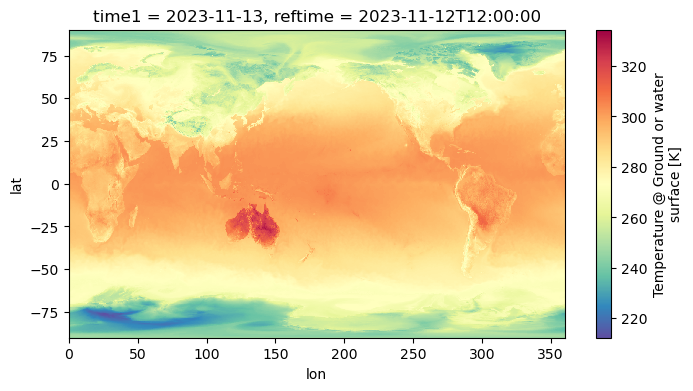
Utilizando Cartopy podemos trabajar con sistemas coordenados de referencia (CRS por sus siglas en ingles Cordinate reference Systems) y diferentes proyecciones. Como ejemplo, trabajaremos con un proyección Mollweide con centro sobre Colombia (285° en longitud aproximadamente).
fig, ax = plt.subplots(
    figsize=(6, 4),
    subplot_kw={"projection": ccrs.Mollweide(central_longitude=285)},
    dpi=150,
)

ds_subset["Temperature_surface"].sel(time1=fecha, method="nearest").plot(
    ax=ax,
    cmap="Spectral_r",
    transform=ccrs.PlateCarree(),
    cbar_kwargs={
        "label": r"$Temperatura \ [°C]$",
        "orientation": "horizontal",
        "aspect": 50,
    },
)
ax.coastlines()
gl = ax.gridlines(
    draw_labels=True, linewidth=1, color="gray", alpha=0.5, linestyle="--"
)
plt.title(f"Temperatura [°C] - {fecha}");
/usr/share/miniconda3/envs/atmoscol2023/lib/python3.11/site-packages/cartopy/io/__init__.py:241: DownloadWarning: Downloading: https://naturalearth.s3.amazonaws.com/110m_physical/ne_110m_coastline.zip
  warnings.warn(f'Downloading: {url}', DownloadWarning)
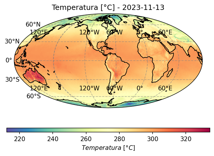
Podemos generar un gráfico para Colombia y sus alrededores de la siguiente manera:
ds_col = ds_subset.sel(lat=slice(20, -10), lon=slice(270, 310))
display(ds_col)
<xarray.Dataset>
Dimensions:                                (time1: 189, lat: 121, lon: 160,
                                            height_above_ground4: 1)
Coordinates:
  * time1                                  (time1) datetime64[ns] 2023-11-05 ...
    reftime                                (time1) datetime64[ns] ...
  * height_above_ground4                   (height_above_ground4) float32 2.0
  * lat                                    (lat) float64 20.0 19.75 ... -10.0
  * lon                                    (lon) float64 270.2 270.4 ... 310.0
Data variables:
    Temperature_surface                    (time1, lat, lon) float32 ...
    Pressure_surface                       (time1, lat, lon) float32 ...
    Precipitation_rate_surface             (time1, lat, lon) float32 ...
    Relative_humidity_height_above_ground  (time1, height_above_ground4, lat, lon) float32 ...
Attributes:
    Originating_or_generating_Center:                                        ...
    Originating_or_generating_Subcenter:                                     ...
    GRIB_table_version:                                                      ...
    Type_of_generating_process:                                              ...
    Analysis_or_forecast_generating_process_identifier_defined_by_originating...
    file_format:                                                             ...
    Conventions:                                                             ...
    history:                                                                 ...
    featureType:                                                             ...
_CoordSysBuilder: ...- time1: 189
- lat: 121
- lon: 160
- height_above_ground4: 1
- time1(time1)datetime64[ns]2023-11-05 ... 2023-11-28T12:00:00
- standard_name :
- time
- long_name :
- GRIB forecast or observation time
- _CoordinateAxisType :
- Time
array(['2023-11-05T00:00:00.000000000', '2023-11-05T03:00:00.000000000', '2023-11-05T06:00:00.000000000', '2023-11-05T09:00:00.000000000', '2023-11-05T12:00:00.000000000', '2023-11-05T15:00:00.000000000', '2023-11-05T18:00:00.000000000', '2023-11-05T21:00:00.000000000', '2023-11-06T00:00:00.000000000', '2023-11-06T03:00:00.000000000', '2023-11-06T06:00:00.000000000', '2023-11-06T09:00:00.000000000', '2023-11-06T12:00:00.000000000', '2023-11-06T15:00:00.000000000', '2023-11-06T18:00:00.000000000', '2023-11-06T21:00:00.000000000', '2023-11-07T00:00:00.000000000', '2023-11-07T03:00:00.000000000', '2023-11-07T06:00:00.000000000', '2023-11-07T09:00:00.000000000', '2023-11-07T12:00:00.000000000', '2023-11-07T15:00:00.000000000', '2023-11-07T18:00:00.000000000', '2023-11-07T21:00:00.000000000', '2023-11-08T00:00:00.000000000', '2023-11-08T03:00:00.000000000', '2023-11-08T06:00:00.000000000', '2023-11-08T09:00:00.000000000', '2023-11-08T12:00:00.000000000', '2023-11-08T15:00:00.000000000', '2023-11-08T18:00:00.000000000', '2023-11-08T21:00:00.000000000', '2023-11-09T00:00:00.000000000', '2023-11-09T03:00:00.000000000', '2023-11-09T06:00:00.000000000', '2023-11-09T09:00:00.000000000', '2023-11-09T12:00:00.000000000', '2023-11-09T15:00:00.000000000', '2023-11-09T18:00:00.000000000', '2023-11-09T21:00:00.000000000', '2023-11-10T00:00:00.000000000', '2023-11-10T03:00:00.000000000', '2023-11-10T06:00:00.000000000', '2023-11-10T09:00:00.000000000', '2023-11-10T12:00:00.000000000', '2023-11-10T15:00:00.000000000', '2023-11-10T18:00:00.000000000', '2023-11-10T21:00:00.000000000', '2023-11-11T00:00:00.000000000', '2023-11-11T03:00:00.000000000', '2023-11-11T06:00:00.000000000', '2023-11-11T09:00:00.000000000', '2023-11-11T12:00:00.000000000', '2023-11-11T15:00:00.000000000', '2023-11-11T18:00:00.000000000', '2023-11-11T21:00:00.000000000', '2023-11-12T00:00:00.000000000', '2023-11-12T03:00:00.000000000', '2023-11-12T06:00:00.000000000', '2023-11-12T09:00:00.000000000', '2023-11-12T12:00:00.000000000', '2023-11-12T15:00:00.000000000', '2023-11-12T18:00:00.000000000', '2023-11-12T21:00:00.000000000', '2023-11-13T00:00:00.000000000', '2023-11-13T03:00:00.000000000', '2023-11-13T06:00:00.000000000', '2023-11-13T09:00:00.000000000', '2023-11-13T12:00:00.000000000', '2023-11-13T15:00:00.000000000', '2023-11-13T18:00:00.000000000', '2023-11-13T21:00:00.000000000', '2023-11-14T00:00:00.000000000', '2023-11-14T03:00:00.000000000', '2023-11-14T06:00:00.000000000', '2023-11-14T09:00:00.000000000', '2023-11-14T12:00:00.000000000', '2023-11-14T15:00:00.000000000', '2023-11-14T18:00:00.000000000', '2023-11-14T21:00:00.000000000', '2023-11-15T00:00:00.000000000', '2023-11-15T03:00:00.000000000', '2023-11-15T06:00:00.000000000', '2023-11-15T09:00:00.000000000', '2023-11-15T12:00:00.000000000', '2023-11-15T15:00:00.000000000', '2023-11-15T18:00:00.000000000', '2023-11-15T21:00:00.000000000', '2023-11-16T00:00:00.000000000', '2023-11-16T03:00:00.000000000', '2023-11-16T06:00:00.000000000', '2023-11-16T09:00:00.000000000', '2023-11-16T12:00:00.000000000', '2023-11-16T15:00:00.000000000', '2023-11-16T18:00:00.000000000', '2023-11-16T21:00:00.000000000', '2023-11-17T00:00:00.000000000', '2023-11-17T03:00:00.000000000', '2023-11-17T06:00:00.000000000', '2023-11-17T09:00:00.000000000', '2023-11-17T12:00:00.000000000', '2023-11-17T15:00:00.000000000', '2023-11-17T18:00:00.000000000', '2023-11-17T21:00:00.000000000', '2023-11-18T00:00:00.000000000', '2023-11-18T03:00:00.000000000', '2023-11-18T06:00:00.000000000', '2023-11-18T09:00:00.000000000', '2023-11-18T12:00:00.000000000', '2023-11-18T15:00:00.000000000', '2023-11-18T18:00:00.000000000', '2023-11-18T21:00:00.000000000', '2023-11-19T00:00:00.000000000', '2023-11-19T03:00:00.000000000', '2023-11-19T06:00:00.000000000', '2023-11-19T09:00:00.000000000', '2023-11-19T12:00:00.000000000', '2023-11-19T15:00:00.000000000', '2023-11-19T18:00:00.000000000', '2023-11-19T21:00:00.000000000', '2023-11-20T00:00:00.000000000', '2023-11-20T03:00:00.000000000', '2023-11-20T06:00:00.000000000', '2023-11-20T09:00:00.000000000', '2023-11-20T12:00:00.000000000', '2023-11-20T15:00:00.000000000', '2023-11-20T18:00:00.000000000', '2023-11-20T21:00:00.000000000', '2023-11-21T00:00:00.000000000', '2023-11-21T03:00:00.000000000', '2023-11-21T06:00:00.000000000', '2023-11-21T09:00:00.000000000', '2023-11-21T12:00:00.000000000', '2023-11-21T15:00:00.000000000', '2023-11-21T18:00:00.000000000', '2023-11-21T21:00:00.000000000', '2023-11-22T00:00:00.000000000', '2023-11-22T03:00:00.000000000', '2023-11-22T06:00:00.000000000', '2023-11-22T09:00:00.000000000', '2023-11-22T12:00:00.000000000', '2023-11-22T15:00:00.000000000', '2023-11-22T18:00:00.000000000', '2023-11-22T21:00:00.000000000', '2023-11-23T00:00:00.000000000', '2023-11-23T03:00:00.000000000', '2023-11-23T06:00:00.000000000', '2023-11-23T09:00:00.000000000', '2023-11-23T12:00:00.000000000', '2023-11-23T15:00:00.000000000', '2023-11-23T18:00:00.000000000', '2023-11-23T21:00:00.000000000', '2023-11-24T00:00:00.000000000', '2023-11-24T03:00:00.000000000', '2023-11-24T06:00:00.000000000', '2023-11-24T09:00:00.000000000', '2023-11-24T12:00:00.000000000', '2023-11-24T15:00:00.000000000', '2023-11-24T18:00:00.000000000', '2023-11-24T21:00:00.000000000', '2023-11-25T00:00:00.000000000', '2023-11-25T03:00:00.000000000', '2023-11-25T06:00:00.000000000', '2023-11-25T09:00:00.000000000', '2023-11-25T12:00:00.000000000', '2023-11-25T15:00:00.000000000', '2023-11-25T18:00:00.000000000', '2023-11-25T21:00:00.000000000', '2023-11-26T00:00:00.000000000', '2023-11-26T03:00:00.000000000', '2023-11-26T06:00:00.000000000', '2023-11-26T09:00:00.000000000', '2023-11-26T12:00:00.000000000', '2023-11-26T15:00:00.000000000', '2023-11-26T18:00:00.000000000', '2023-11-26T21:00:00.000000000', '2023-11-27T00:00:00.000000000', '2023-11-27T03:00:00.000000000', '2023-11-27T06:00:00.000000000', '2023-11-27T09:00:00.000000000', '2023-11-27T12:00:00.000000000', '2023-11-27T15:00:00.000000000', '2023-11-27T18:00:00.000000000', '2023-11-27T21:00:00.000000000', '2023-11-28T00:00:00.000000000', '2023-11-28T03:00:00.000000000', '2023-11-28T06:00:00.000000000', '2023-11-28T09:00:00.000000000', '2023-11-28T12:00:00.000000000'], dtype='datetime64[ns]') - reftime(time1)datetime64[ns]...
- standard_name :
- forecast_reference_time
- long_name :
- GRIB reference time
- _CoordinateAxisType :
- RunTime
[189 values with dtype=datetime64[ns]]
- height_above_ground4(height_above_ground4)float322.0
- units :
- m
- long_name :
- Specified height level above ground
- positive :
- up
- Grib_level_type :
- 103
- datum :
- ground
- _CoordinateAxisType :
- Height
- _CoordinateZisPositive :
- up
array([2.], dtype=float32)
- lat(lat)float6420.0 19.75 19.5 ... -9.75 -10.0
array([ 20. , 19.75, 19.5 , 19.25, 19. , 18.75, 18.5 , 18.25, 18. , 17.75, 17.5 , 17.25, 17. , 16.75, 16.5 , 16.25, 16. , 15.75, 15.5 , 15.25, 15. , 14.75, 14.5 , 14.25, 14. , 13.75, 13.5 , 13.25, 13. , 12.75, 12.5 , 12.25, 12. , 11.75, 11.5 , 11.25, 11. , 10.75, 10.5 , 10.25, 10. , 9.75, 9.5 , 9.25, 9. , 8.75, 8.5 , 8.25, 8. , 7.75, 7.5 , 7.25, 7. , 6.75, 6.5 , 6.25, 6. , 5.75, 5.5 , 5.25, 5. , 4.75, 4.5 , 4.25, 4. , 3.75, 3.5 , 3.25, 3. , 2.75, 2.5 , 2.25, 2. , 1.75, 1.5 , 1.25, 1. , 0.75, 0.5 , 0.25, 0. , -0.25, -0.5 , -0.75, -1. , -1.25, -1.5 , -1.75, -2. , -2.25, -2.5 , -2.75, -3. , -3.25, -3.5 , -3.75, -4. , -4.25, -4.5 , -4.75, -5. , -5.25, -5.5 , -5.75, -6. , -6.25, -6.5 , -6.75, -7. , -7.25, -7.5 , -7.75, -8. , -8.25, -8.5 , -8.75, -9. , -9.25, -9.5 , -9.75, -10. ]) - lon(lon)float64270.2 270.4 270.7 ... 309.7 310.0
array([270.18763 , 270.437804, 270.687978, 270.938151, 271.188325, 271.438499,
       271.688673, 271.938846, 272.18902 , 272.439194, 272.689368, 272.939541,
       273.189715, 273.439889, 273.690063, 273.940236, 274.19041 , 274.440584,
       274.690757, 274.940931, 275.191105, 275.441279, 275.691452, 275.941626,
       276.1918  , 276.441974, 276.692147, 276.942321, 277.192495, 277.442669,
       277.692842, 277.943016, 278.19319 , 278.443363, 278.693537, 278.943711,
       279.193885, 279.444058, 279.694232, 279.944406, 280.19458 , 280.444753,
       280.694927, 280.945101, 281.195274, 281.445448, 281.695622, 281.945796,
       282.195969, 282.446143, 282.696317, 282.946491, 283.196664, 283.446838,
       283.697012, 283.947186, 284.197359, 284.447533, 284.697707, 284.94788 ,
       285.198054, 285.448228, 285.698402, 285.948575, 286.198749, 286.448923,
       286.699097, 286.94927 , 287.199444, 287.449618, 287.699792, 287.949965,
       288.200139, 288.450313, 288.700486, 288.95066 , 289.200834, 289.451008,
       289.701181, 289.951355, 290.201529, 290.451703, 290.701876, 290.95205 ,
       291.202224, 291.452397, 291.702571, 291.952745, 292.202919, 292.453092,
       292.703266, 292.95344 , 293.203614, 293.453787, 293.703961, 293.954135,
       294.204309, 294.454482, 294.704656, 294.95483 , 295.205003, 295.455177,
       295.705351, 295.955525, 296.205698, 296.455872, 296.706046, 296.95622 ,
       297.206393, 297.456567, 297.706741, 297.956915, 298.207088, 298.457262,
       298.707436, 298.957609, 299.207783, 299.457957, 299.708131, 299.958304,
       300.208478, 300.458652, 300.708826, 300.958999, 301.209173, 301.459347,
       301.709521, 301.959694, 302.209868, 302.460042, 302.710215, 302.960389,
       303.210563, 303.460737, 303.71091 , 303.961084, 304.211258, 304.461432,
       304.711605, 304.961779, 305.211953, 305.462126, 305.7123  , 305.962474,
       306.212648, 306.462821, 306.712995, 306.963169, 307.213343, 307.463516,
       307.71369 , 307.963864, 308.214038, 308.464211, 308.714385, 308.964559,
       309.214732, 309.464906, 309.71508 , 309.965254])
- Temperature_surface(time1, lat, lon)float32...
- long_name :
- Temperature @ Ground or water surface
- units :
- K
- abbreviation :
- TMP
- grid_mapping :
- LatLon_Projection
- Grib_Variable_Id :
- VAR_7-0--1-0_L1
- Grib2_Parameter :
- [0 0 0]
- Grib2_Parameter_Discipline :
- Meteorological products
- Grib2_Parameter_Category :
- Temperature
- Grib2_Parameter_Name :
- Temperature
- Grib2_Level_Type :
- 1
- Grib2_Level_Desc :
- Ground or water surface
- Grib2_Generating_Process_Type :
- Forecast
- Grib2_Statistical_Process_Type :
- UnknownStatType--1
[3659040 values with dtype=float32]
- Pressure_surface(time1, lat, lon)float32...
- long_name :
- Pressure @ Ground or water surface
- units :
- Pa
- abbreviation :
- PRES
- grid_mapping :
- LatLon_Projection
- Grib_Variable_Id :
- VAR_7-0--1-0_L1
- Grib2_Parameter :
- [0 3 0]
- Grib2_Parameter_Discipline :
- Meteorological products
- Grib2_Parameter_Category :
- Mass
- Grib2_Parameter_Name :
- Pressure
- Grib2_Level_Type :
- 1
- Grib2_Level_Desc :
- Ground or water surface
- Grib2_Generating_Process_Type :
- Forecast
- Grib2_Statistical_Process_Type :
- UnknownStatType--1
[3659040 values with dtype=float32]
- Precipitation_rate_surface(time1, lat, lon)float32...
- long_name :
- Precipitation rate @ Ground or water surface
- units :
- kg.m-2.s-1
- abbreviation :
- PRATE
- grid_mapping :
- LatLon_Projection
- Grib_Variable_Id :
- VAR_7-0--1-7_L1
- Grib2_Parameter :
- [0 1 7]
- Grib2_Parameter_Discipline :
- Meteorological products
- Grib2_Parameter_Category :
- Moisture
- Grib2_Parameter_Name :
- Precipitation rate
- Grib2_Level_Type :
- 1
- Grib2_Level_Desc :
- Ground or water surface
- Grib2_Generating_Process_Type :
- Forecast
- Grib2_Statistical_Process_Type :
- UnknownStatType--1
[3659040 values with dtype=float32]
- Relative_humidity_height_above_ground(time1, height_above_ground4, lat, lon)float32...
- long_name :
- Relative humidity @ Specified height level above ground
- units :
- %
- abbreviation :
- RH
- grid_mapping :
- LatLon_Projection
- Grib_Variable_Id :
- VAR_7-0--1-1_L103
- Grib2_Parameter :
- [0 1 1]
- Grib2_Parameter_Discipline :
- Meteorological products
- Grib2_Parameter_Category :
- Moisture
- Grib2_Parameter_Name :
- Relative humidity
- Grib2_Level_Type :
- 103
- Grib2_Level_Desc :
- Specified height level above ground
- Grib2_Generating_Process_Type :
- Forecast
- Grib2_Statistical_Process_Type :
- UnknownStatType--1
[3659040 values with dtype=float32]
- time1PandasIndex
PandasIndex(DatetimeIndex(['2023-11-05 00:00:00', '2023-11-05 03:00:00', '2023-11-05 06:00:00', '2023-11-05 09:00:00', '2023-11-05 12:00:00', '2023-11-05 15:00:00', '2023-11-05 18:00:00', '2023-11-05 21:00:00', '2023-11-06 00:00:00', '2023-11-06 03:00:00', ... '2023-11-27 09:00:00', '2023-11-27 12:00:00', '2023-11-27 15:00:00', '2023-11-27 18:00:00', '2023-11-27 21:00:00', '2023-11-28 00:00:00', '2023-11-28 03:00:00', '2023-11-28 06:00:00', '2023-11-28 09:00:00', '2023-11-28 12:00:00'], dtype='datetime64[ns]', name='time1', length=189, freq=None)) - height_above_ground4PandasIndex
PandasIndex(Index([2.0], dtype='>f4', name='height_above_ground4'))
- latPandasIndex
PandasIndex(Index([ 20.0, 19.75, 19.5, 19.25, 19.0, 18.75, 18.5, 18.25, 18.0, 17.75, ... -7.75, -8.0, -8.25, -8.5, -8.75, -9.0, -9.25, -9.5, -9.75, -10.0], dtype='float64', name='lat', length=121)) - lonPandasIndex
PandasIndex(Index([ 270.1876302988186,  270.4378040305768,  270.6879777623349,
        270.9381514940931, 271.18832522585126, 271.43849895760945,
        271.6886726893676,  271.9388464211258,  272.1890201528839,
       272.43919388464207,
       ...
       307.71369006254344,  307.9638637943016, 308.21403752605977,
        308.4642112578179, 308.71438498957605, 308.96455872133424,
        309.2147324530924,  309.4649061848506,  309.7150799166087,
        309.9652536483669],
      dtype='float64', name='lon', length=160))
- Originating_or_generating_Center :
- US National Weather Service, National Centres for Environmental Prediction (NCEP)
- Originating_or_generating_Subcenter :
- 0
- GRIB_table_version :
- 2,1
- Type_of_generating_process :
- Forecast
- Analysis_or_forecast_generating_process_identifier_defined_by_originating_centre :
- Analysis from GFS (Global Forecast System)
- file_format :
- GRIB-2
- Conventions :
- CF-1.6
- history :
- Read using CDM IOSP GribCollection v3
- featureType :
- GRID
- _CoordSysBuilder :
- ucar.nc2.dataset.conv.CF1Convention
De igual modo podemos visualizar los datos usando contour y contourf. A continuación, podemos observar los gráficos de la temperatura, presión, precipitación y humedad relativa
# Creación del "lienzo"
fig, ax = plt.subplots(
    figsize=(7, 4),
    subplot_kw={"projection": ccrs.PlateCarree(central_longitude=285)},
    dpi=150,
)

# Grafico de variables
# (ds_col.Pressure_surface.sel(time1=f"{fecha} 12:00") / 100).plot.contour(ax=ax, transform=ccrs.PlateCarree(), cmap='viridis_r',
#                                              linewidths=0.5,
#                                             levels=np.arange(500, 1000, 100))
# (ds_col.Temperature_surface.sel(time1=f"{fecha} 12:00") - 273.15).plot.contourf(ax=ax, cmap='Spectral_r', transform=ccrs.PlateCarree(),
#                                          levels=np.arange(0, 35, 1))
ds_col.Relative_humidity_height_above_ground.sel(time1=f"{fecha} 12:00").isel(
    height_above_ground4=0
).plot.contourf(
    ax=ax, cmap="viridis", transform=ccrs.PlateCarree(), levels=np.arange(0, 101, 10)
)

# (ds_col.Precipitation_rate_surface.sel(time=f"{fecha} 12:00") * 86400).plot.contourf(ax=ax,
#                                                           transform=ccrs.PlateCarree(),
#                                                           levels=np.arange(0, 50, 1))

# Adicionamos lineas costeras y división entre países
ax.coastlines()
ax.add_feature(cf.BORDERS)

# Agregar las líneas de reticula
gl = ax.gridlines(
    draw_labels=True, linewidth=1, color="gray", alpha=0.5, linestyle="--"
)
gl.xlabels_top = False
gl.ylabels_right = False
plt.title(
    f"{to_datetime(ds_col.sel(time1=f'{fecha} 12:00').time1.values):%Y-%m-%d %H%M} UTC"
);
/usr/share/miniconda3/envs/atmoscol2023/lib/python3.11/site-packages/cartopy/mpl/gridliner.py:451: UserWarning: The .xlabels_top attribute is deprecated. Please use .top_labels to toggle visibility instead.
  warnings.warn('The .xlabels_top attribute is deprecated. Please '
/usr/share/miniconda3/envs/atmoscol2023/lib/python3.11/site-packages/cartopy/mpl/gridliner.py:487: UserWarning: The .ylabels_right attribute is deprecated. Please use .right_labels to toggle visibility instead.
  warnings.warn('The .ylabels_right attribute is deprecated. Please '
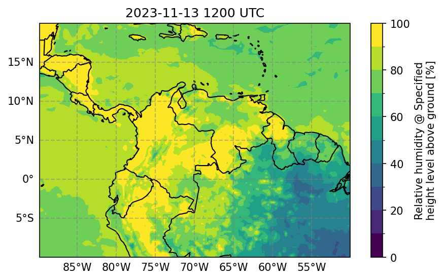
Podemos gener series de tiempo con los valores pronosticados para una ubicacion en particular. Utilicemos la ubicación de la Universidad del Quindio como ejemplo: lat=4.54 y lon=-75.68.
ds_uniq = ds_col.sel(lat=4.54, lon=360 - 75.0, method="nearest")
ds_uniq
<xarray.Dataset>
Dimensions:                                (time1: 189, height_above_ground4: 1)
Coordinates:
  * time1                                  (time1) datetime64[ns] 2023-11-05 ...
    reftime                                (time1) datetime64[ns] ...
  * height_above_ground4                   (height_above_ground4) float32 2.0
    lat                                    float64 4.5
    lon                                    float64 284.9
Data variables:
    Temperature_surface                    (time1) float32 ...
    Pressure_surface                       (time1) float32 ...
    Precipitation_rate_surface             (time1) float32 ...
    Relative_humidity_height_above_ground  (time1, height_above_ground4) float32 ...
Attributes:
    Originating_or_generating_Center:                                        ...
    Originating_or_generating_Subcenter:                                     ...
    GRIB_table_version:                                                      ...
    Type_of_generating_process:                                              ...
    Analysis_or_forecast_generating_process_identifier_defined_by_originating...
    file_format:                                                             ...
    Conventions:                                                             ...
    history:                                                                 ...
    featureType:                                                             ...
_CoordSysBuilder: ...- time1: 189
- height_above_ground4: 1
- time1(time1)datetime64[ns]2023-11-05 ... 2023-11-28T12:00:00
- standard_name :
- time
- long_name :
- GRIB forecast or observation time
- _CoordinateAxisType :
- Time
array(['2023-11-05T00:00:00.000000000', '2023-11-05T03:00:00.000000000', '2023-11-05T06:00:00.000000000', '2023-11-05T09:00:00.000000000', '2023-11-05T12:00:00.000000000', '2023-11-05T15:00:00.000000000', '2023-11-05T18:00:00.000000000', '2023-11-05T21:00:00.000000000', '2023-11-06T00:00:00.000000000', '2023-11-06T03:00:00.000000000', '2023-11-06T06:00:00.000000000', '2023-11-06T09:00:00.000000000', '2023-11-06T12:00:00.000000000', '2023-11-06T15:00:00.000000000', '2023-11-06T18:00:00.000000000', '2023-11-06T21:00:00.000000000', '2023-11-07T00:00:00.000000000', '2023-11-07T03:00:00.000000000', '2023-11-07T06:00:00.000000000', '2023-11-07T09:00:00.000000000', '2023-11-07T12:00:00.000000000', '2023-11-07T15:00:00.000000000', '2023-11-07T18:00:00.000000000', '2023-11-07T21:00:00.000000000', '2023-11-08T00:00:00.000000000', '2023-11-08T03:00:00.000000000', '2023-11-08T06:00:00.000000000', '2023-11-08T09:00:00.000000000', '2023-11-08T12:00:00.000000000', '2023-11-08T15:00:00.000000000', '2023-11-08T18:00:00.000000000', '2023-11-08T21:00:00.000000000', '2023-11-09T00:00:00.000000000', '2023-11-09T03:00:00.000000000', '2023-11-09T06:00:00.000000000', '2023-11-09T09:00:00.000000000', '2023-11-09T12:00:00.000000000', '2023-11-09T15:00:00.000000000', '2023-11-09T18:00:00.000000000', '2023-11-09T21:00:00.000000000', '2023-11-10T00:00:00.000000000', '2023-11-10T03:00:00.000000000', '2023-11-10T06:00:00.000000000', '2023-11-10T09:00:00.000000000', '2023-11-10T12:00:00.000000000', '2023-11-10T15:00:00.000000000', '2023-11-10T18:00:00.000000000', '2023-11-10T21:00:00.000000000', '2023-11-11T00:00:00.000000000', '2023-11-11T03:00:00.000000000', '2023-11-11T06:00:00.000000000', '2023-11-11T09:00:00.000000000', '2023-11-11T12:00:00.000000000', '2023-11-11T15:00:00.000000000', '2023-11-11T18:00:00.000000000', '2023-11-11T21:00:00.000000000', '2023-11-12T00:00:00.000000000', '2023-11-12T03:00:00.000000000', '2023-11-12T06:00:00.000000000', '2023-11-12T09:00:00.000000000', '2023-11-12T12:00:00.000000000', '2023-11-12T15:00:00.000000000', '2023-11-12T18:00:00.000000000', '2023-11-12T21:00:00.000000000', '2023-11-13T00:00:00.000000000', '2023-11-13T03:00:00.000000000', '2023-11-13T06:00:00.000000000', '2023-11-13T09:00:00.000000000', '2023-11-13T12:00:00.000000000', '2023-11-13T15:00:00.000000000', '2023-11-13T18:00:00.000000000', '2023-11-13T21:00:00.000000000', '2023-11-14T00:00:00.000000000', '2023-11-14T03:00:00.000000000', '2023-11-14T06:00:00.000000000', '2023-11-14T09:00:00.000000000', '2023-11-14T12:00:00.000000000', '2023-11-14T15:00:00.000000000', '2023-11-14T18:00:00.000000000', '2023-11-14T21:00:00.000000000', '2023-11-15T00:00:00.000000000', '2023-11-15T03:00:00.000000000', '2023-11-15T06:00:00.000000000', '2023-11-15T09:00:00.000000000', '2023-11-15T12:00:00.000000000', '2023-11-15T15:00:00.000000000', '2023-11-15T18:00:00.000000000', '2023-11-15T21:00:00.000000000', '2023-11-16T00:00:00.000000000', '2023-11-16T03:00:00.000000000', '2023-11-16T06:00:00.000000000', '2023-11-16T09:00:00.000000000', '2023-11-16T12:00:00.000000000', '2023-11-16T15:00:00.000000000', '2023-11-16T18:00:00.000000000', '2023-11-16T21:00:00.000000000', '2023-11-17T00:00:00.000000000', '2023-11-17T03:00:00.000000000', '2023-11-17T06:00:00.000000000', '2023-11-17T09:00:00.000000000', '2023-11-17T12:00:00.000000000', '2023-11-17T15:00:00.000000000', '2023-11-17T18:00:00.000000000', '2023-11-17T21:00:00.000000000', '2023-11-18T00:00:00.000000000', '2023-11-18T03:00:00.000000000', '2023-11-18T06:00:00.000000000', '2023-11-18T09:00:00.000000000', '2023-11-18T12:00:00.000000000', '2023-11-18T15:00:00.000000000', '2023-11-18T18:00:00.000000000', '2023-11-18T21:00:00.000000000', '2023-11-19T00:00:00.000000000', '2023-11-19T03:00:00.000000000', '2023-11-19T06:00:00.000000000', '2023-11-19T09:00:00.000000000', '2023-11-19T12:00:00.000000000', '2023-11-19T15:00:00.000000000', '2023-11-19T18:00:00.000000000', '2023-11-19T21:00:00.000000000', '2023-11-20T00:00:00.000000000', '2023-11-20T03:00:00.000000000', '2023-11-20T06:00:00.000000000', '2023-11-20T09:00:00.000000000', '2023-11-20T12:00:00.000000000', '2023-11-20T15:00:00.000000000', '2023-11-20T18:00:00.000000000', '2023-11-20T21:00:00.000000000', '2023-11-21T00:00:00.000000000', '2023-11-21T03:00:00.000000000', '2023-11-21T06:00:00.000000000', '2023-11-21T09:00:00.000000000', '2023-11-21T12:00:00.000000000', '2023-11-21T15:00:00.000000000', '2023-11-21T18:00:00.000000000', '2023-11-21T21:00:00.000000000', '2023-11-22T00:00:00.000000000', '2023-11-22T03:00:00.000000000', '2023-11-22T06:00:00.000000000', '2023-11-22T09:00:00.000000000', '2023-11-22T12:00:00.000000000', '2023-11-22T15:00:00.000000000', '2023-11-22T18:00:00.000000000', '2023-11-22T21:00:00.000000000', '2023-11-23T00:00:00.000000000', '2023-11-23T03:00:00.000000000', '2023-11-23T06:00:00.000000000', '2023-11-23T09:00:00.000000000', '2023-11-23T12:00:00.000000000', '2023-11-23T15:00:00.000000000', '2023-11-23T18:00:00.000000000', '2023-11-23T21:00:00.000000000', '2023-11-24T00:00:00.000000000', '2023-11-24T03:00:00.000000000', '2023-11-24T06:00:00.000000000', '2023-11-24T09:00:00.000000000', '2023-11-24T12:00:00.000000000', '2023-11-24T15:00:00.000000000', '2023-11-24T18:00:00.000000000', '2023-11-24T21:00:00.000000000', '2023-11-25T00:00:00.000000000', '2023-11-25T03:00:00.000000000', '2023-11-25T06:00:00.000000000', '2023-11-25T09:00:00.000000000', '2023-11-25T12:00:00.000000000', '2023-11-25T15:00:00.000000000', '2023-11-25T18:00:00.000000000', '2023-11-25T21:00:00.000000000', '2023-11-26T00:00:00.000000000', '2023-11-26T03:00:00.000000000', '2023-11-26T06:00:00.000000000', '2023-11-26T09:00:00.000000000', '2023-11-26T12:00:00.000000000', '2023-11-26T15:00:00.000000000', '2023-11-26T18:00:00.000000000', '2023-11-26T21:00:00.000000000', '2023-11-27T00:00:00.000000000', '2023-11-27T03:00:00.000000000', '2023-11-27T06:00:00.000000000', '2023-11-27T09:00:00.000000000', '2023-11-27T12:00:00.000000000', '2023-11-27T15:00:00.000000000', '2023-11-27T18:00:00.000000000', '2023-11-27T21:00:00.000000000', '2023-11-28T00:00:00.000000000', '2023-11-28T03:00:00.000000000', '2023-11-28T06:00:00.000000000', '2023-11-28T09:00:00.000000000', '2023-11-28T12:00:00.000000000'], dtype='datetime64[ns]') - reftime(time1)datetime64[ns]...
- standard_name :
- forecast_reference_time
- long_name :
- GRIB reference time
- _CoordinateAxisType :
- RunTime
[189 values with dtype=datetime64[ns]]
- height_above_ground4(height_above_ground4)float322.0
- units :
- m
- long_name :
- Specified height level above ground
- positive :
- up
- Grib_level_type :
- 103
- datum :
- ground
- _CoordinateAxisType :
- Height
- _CoordinateZisPositive :
- up
array([2.], dtype=float32)
- lat()float644.5
array(4.5)
- lon()float64284.9
array(284.94788047)
- Temperature_surface(time1)float32...
- long_name :
- Temperature @ Ground or water surface
- units :
- K
- abbreviation :
- TMP
- grid_mapping :
- LatLon_Projection
- Grib_Variable_Id :
- VAR_7-0--1-0_L1
- Grib2_Parameter :
- [0 0 0]
- Grib2_Parameter_Discipline :
- Meteorological products
- Grib2_Parameter_Category :
- Temperature
- Grib2_Parameter_Name :
- Temperature
- Grib2_Level_Type :
- 1
- Grib2_Level_Desc :
- Ground or water surface
- Grib2_Generating_Process_Type :
- Forecast
- Grib2_Statistical_Process_Type :
- UnknownStatType--1
[189 values with dtype=float32]
- Pressure_surface(time1)float32...
- long_name :
- Pressure @ Ground or water surface
- units :
- Pa
- abbreviation :
- PRES
- grid_mapping :
- LatLon_Projection
- Grib_Variable_Id :
- VAR_7-0--1-0_L1
- Grib2_Parameter :
- [0 3 0]
- Grib2_Parameter_Discipline :
- Meteorological products
- Grib2_Parameter_Category :
- Mass
- Grib2_Parameter_Name :
- Pressure
- Grib2_Level_Type :
- 1
- Grib2_Level_Desc :
- Ground or water surface
- Grib2_Generating_Process_Type :
- Forecast
- Grib2_Statistical_Process_Type :
- UnknownStatType--1
[189 values with dtype=float32]
- Precipitation_rate_surface(time1)float32...
- long_name :
- Precipitation rate @ Ground or water surface
- units :
- kg.m-2.s-1
- abbreviation :
- PRATE
- grid_mapping :
- LatLon_Projection
- Grib_Variable_Id :
- VAR_7-0--1-7_L1
- Grib2_Parameter :
- [0 1 7]
- Grib2_Parameter_Discipline :
- Meteorological products
- Grib2_Parameter_Category :
- Moisture
- Grib2_Parameter_Name :
- Precipitation rate
- Grib2_Level_Type :
- 1
- Grib2_Level_Desc :
- Ground or water surface
- Grib2_Generating_Process_Type :
- Forecast
- Grib2_Statistical_Process_Type :
- UnknownStatType--1
[189 values with dtype=float32]
- Relative_humidity_height_above_ground(time1, height_above_ground4)float32...
- long_name :
- Relative humidity @ Specified height level above ground
- units :
- %
- abbreviation :
- RH
- grid_mapping :
- LatLon_Projection
- Grib_Variable_Id :
- VAR_7-0--1-1_L103
- Grib2_Parameter :
- [0 1 1]
- Grib2_Parameter_Discipline :
- Meteorological products
- Grib2_Parameter_Category :
- Moisture
- Grib2_Parameter_Name :
- Relative humidity
- Grib2_Level_Type :
- 103
- Grib2_Level_Desc :
- Specified height level above ground
- Grib2_Generating_Process_Type :
- Forecast
- Grib2_Statistical_Process_Type :
- UnknownStatType--1
[189 values with dtype=float32]
- time1PandasIndex
PandasIndex(DatetimeIndex(['2023-11-05 00:00:00', '2023-11-05 03:00:00', '2023-11-05 06:00:00', '2023-11-05 09:00:00', '2023-11-05 12:00:00', '2023-11-05 15:00:00', '2023-11-05 18:00:00', '2023-11-05 21:00:00', '2023-11-06 00:00:00', '2023-11-06 03:00:00', ... '2023-11-27 09:00:00', '2023-11-27 12:00:00', '2023-11-27 15:00:00', '2023-11-27 18:00:00', '2023-11-27 21:00:00', '2023-11-28 00:00:00', '2023-11-28 03:00:00', '2023-11-28 06:00:00', '2023-11-28 09:00:00', '2023-11-28 12:00:00'], dtype='datetime64[ns]', name='time1', length=189, freq=None)) - height_above_ground4PandasIndex
PandasIndex(Index([2.0], dtype='>f4', name='height_above_ground4'))
- Originating_or_generating_Center :
- US National Weather Service, National Centres for Environmental Prediction (NCEP)
- Originating_or_generating_Subcenter :
- 0
- GRIB_table_version :
- 2,1
- Type_of_generating_process :
- Forecast
- Analysis_or_forecast_generating_process_identifier_defined_by_originating_centre :
- Analysis from GFS (Global Forecast System)
- file_format :
- GRIB-2
- Conventions :
- CF-1.6
- history :
- Read using CDM IOSP GribCollection v3
- featureType :
- GRID
- _CoordSysBuilder :
- ucar.nc2.dataset.conv.CF1Convention
fig, (ax, ax1, ax2, ax3) = plt.subplots(4, 1, figsize=(10, 6), sharex=True)
(ds_uniq.Pressure_surface / 100).plot(ax=ax)
ax.set_title("")
ax.set_xlabel("")
ax.set_ylabel("Press [hPa]")
(ds_uniq.Temperature_surface - 273.15).plot(ax=ax1)
ax1.set_title("")
ax1.set_xlabel("")
ax1.set_ylabel("Temp [°C]")
(ds_uniq.Precipitation_rate_surface * 86400).plot(ax=ax2)
ax2.set_title("")
ax2.set_xlabel("")
ax2.set_ylabel("RR [mmhr-1]")
ds_uniq.Relative_humidity_height_above_ground.isel(height_above_ground4=0).plot(ax=ax3)
ax3.set_title("")
ax3.set_xlabel("")
ax3.set_ylabel("HR [%]")
Text(0, 0.5, 'HR [%]')
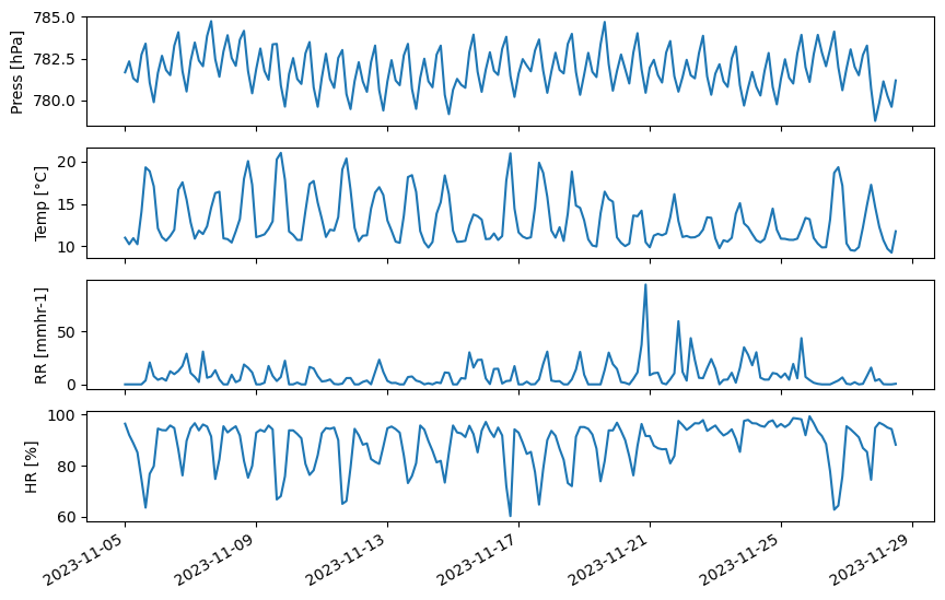
Otras variables disponibles en el modelo GFS pueden ser gráficadas.
Conclusiones
En este cuadernillo aprendimos a consultar datos provenientes del modelo Global Forecast System usando la librería Siphon disponibles en el servidor Thredds de la NCAR. Aprendimos a generar gráficos espaciales y series temporales de pronósticos para múltiples variables usando Xarray, Cartopy y Matplotlib.