ESGF Compute Function Service Demo

Overview

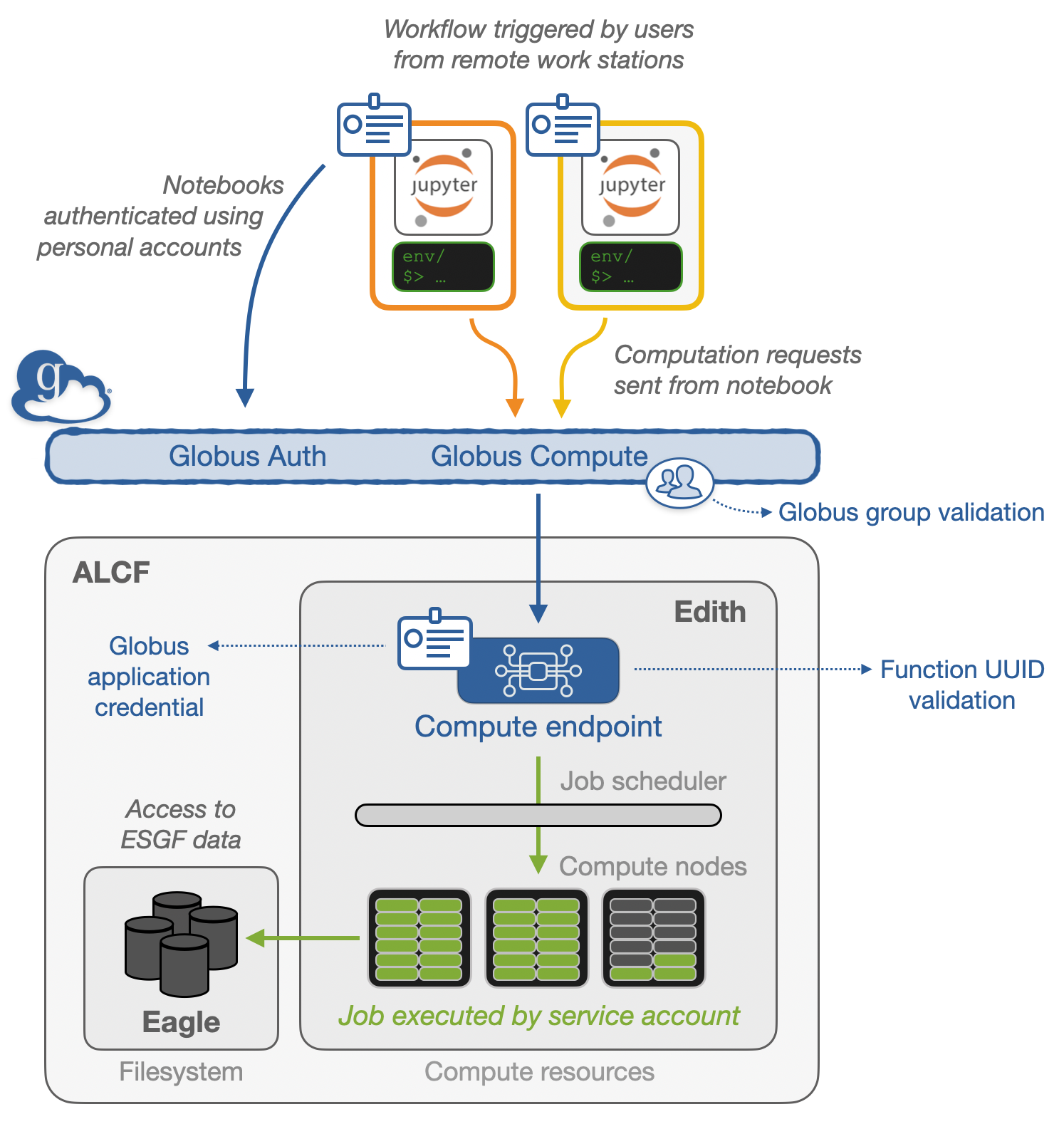
Prior to this demo, a globus-compute function was registered at the Argonne Leadership Computing Facility (ALCF), which has direct file-access to several petabytes of ESGF data. esgf-compute-diagram

Prerequisites

Concepts	Importance	Notes
Intro to Xarray	Necessary
Globus Compute Workflows	Necessary	Understanding of globus compute workflows
Understanding of NetCDF	Helpful	Familiarity with metadata structure
hvPlot with Xarray	Helpful	Familiarity with plotting with Xarray and hvPlot

Time to learn: 15 minutes

Imports

We need to import a few libraries to visualize the output of our data! The rest of the libraries are installed and run on where we defined the function (ALCF).

# Import packages to help with data visualization
import holoviews as hv
import hvplot
import hvplot.xarray
hv.extension('bokeh')

# Import Globus tools
from globus_compute_sdk import Executor

Visualize the Dataset Locally

Now that we have the dataset, we can use holoviz tools to create an interactive plot!

def plot_enso(ds):
    el_nino = ds.hvplot.area(x="time", y2='tos_gt_04', y='el_nino_threshold', color='red', hover=False)
    el_nino_label = hv.Text(ds.isel(time=40).time.values, 2, 'El Niño').opts(text_color='red',)

    # Create the La Niña area graphs
    la_nina = ds.hvplot.area(x="time", y2='tos_lt_04', y='la_nina_threshold', color='blue', hover=False)
    la_nina_label = hv.Text(ds.isel(time=-40).time.values, -2, 'La Niña').opts(text_color='blue')

    # Plot a timeseries of the ENSO 3.4 index
    enso = ds.tos.hvplot(x='time', line_width=0.5, color='k', xlabel='Year', ylabel='ENSO 3.4 Index')

    # Combine all the plots into a single plot
    return (el_nino_label * la_nina_label * el_nino * la_nina * enso).opts(title=f'{ds.attrs["model"]} {ds.attrs["source_id"]} \n Ensemble Member: {ds.attrs["variant_label"]}')

plot_enso(ds)

What was in the `49cd1ee0-2c4c-45f1-ab78-c4557fa25aa3` function??

Below is the exact code that was registered at ALCF. If you are interested in writing your own compute functions, please review the Globus Compute with ENSO Notebook

Show code cell source Hide code cell source

def run_plot_enso(source_id):
    from intake_esgf.exceptions import NoSearchResults
    import numpy as np
    import matplotlib.pyplot as plt
    from intake_esgf import ESGFCatalog
    import xarray as xr
    import cf_xarray
    import warnings
    warnings.filterwarnings("ignore")

    # List of available source ids
    valid_source_id = [
        'ACCESS-ESM1-5', 'EC-Earth3-CC', 'MPI-ESM1-2-LR', 'CanESM5',
        'MIROC6', 'EC-Earth3', 'CESM2', 'EC-Earth3-Veg', 'NorCPM1'
    ]

    # Validate user input
    if not isinstance(source_id, str):
        raise ValueError("Source ID should be a string.")
    if not source_id in valid_source_id:
        raise NoSearchResults("Please use one of the following: "+", ".join(valid_source_id))

    def search_esgf(source_id):

        # Search and load the ocean surface temperature (tos)
        cat = ESGFCatalog(esgf1_indices="anl-dev")
        cat.search(
            activity_id="CMIP",
            experiment_id="historical",
            variable_id=["tos"],
            source_id=source_id,
            member_id='r1i1p1f1',
            grid_label="gn",
            table_id="Omon",
        )
        try:
            tos_ds = cat.to_dataset_dict()["tos"]
        except ValueError:
            print(f"Issue with {institution_id} dataset")

        return tos_ds

    def calculate_enso(ds):

        # Subset the El Nino 3.4 index region
        dso = ds.where(
        (ds.cf["latitude"] < 5) & (ds.cf["latitude"] > -5) & (ds.cf["longitude"] > 190) & (ds.cf["longitude"] < 240), drop=True
        )

        # Calculate the monthly means
        gb = dso.tos.groupby('time.month')

        # Subtract the monthly averages, returning the anomalies
        tos_nino34_anom = gb - gb.mean(dim='time')

        # Determine the non-time dimensions and average using these
        non_time_dims = set(tos_nino34_anom.dims)
        non_time_dims.remove(ds.tos.cf["T"].name)
        weighted_average = tos_nino34_anom.weighted(ds["areacello"].fillna(0)).mean(dim=list(non_time_dims))

        # Calculate the rolling average
        rolling_average = weighted_average.rolling(time=5, center=True).mean()
        std_dev = weighted_average.std()
        return rolling_average / std_dev

    def add_enso_thresholds(da, threshold=0.4):

        # Conver the xr.DataArray into an xr.Dataset
        ds = da.to_dataset()

        # Cleanup the time and use the thresholds
        try:
            ds["time"]= ds.indexes["time"].to_datetimeindex()
        except:
            pass
        ds["tos_gt_04"] = ("time", ds.tos.where(ds.tos >= threshold, threshold).data)
        ds["tos_lt_04"] = ("time", ds.tos.where(ds.tos <= -threshold, -threshold).data)

        # Add fields for the thresholds
        ds["el_nino_threshold"] = ("time", np.zeros_like(ds.tos) + threshold)
        ds["la_nina_threshold"] = ("time", np.zeros_like(ds.tos) - threshold)

        return ds
    
    ds = search_esgf(source_id)
    enso_index = add_enso_thresholds(calculate_enso(ds).compute())
    enso_index.attrs = ds.attrs
    enso_index.attrs["model"] = source_id

    return enso_index

Summary

Within this demonstration, we remotely triggered a globus-compute function which read, aggregated, and computed ENSO on datasets located on an HPC system. The computations were all done on the server side, with visualization being the only task done locally.

What’s next?

Some existing questions still exist! Mainly:

Where do define these functions? How do we ensure these are safe to run?
How do we request “service” accounts on other HPC/cloud facilities?
What other functions, outside of the typical WPS services, can we define?
What other use-cases could this support (ex. kerchunk or zarr creation)?

ESGF Compute Function Service Demo

Overview

Prerequisites

Imports

Remotely Execute + Access ENSO Data from CMIP6

Create Globus compute executor

Pass in the `source_id` of Interest

Visualize the Dataset Locally

What was in the `49cd1ee0-2c4c-45f1-ab78-c4557fa25aa3` function??

Summary

What’s next?

Resources and references

ESGF Compute Function Service Demo

Overview

Prerequisites

Imports

Remotely Execute + Access ENSO Data from CMIP6

Create Globus compute executor

Pass in the source_id of Interest

Visualize the Dataset Locally

What was in the 49cd1ee0-2c4c-45f1-ab78-c4557fa25aa3 function??

Summary

What’s next?

Resources and references

Pass in the `source_id` of Interest

What was in the `49cd1ee0-2c4c-45f1-ab78-c4557fa25aa3` function??