Unstructured Grids Overview
The goal of this notebook is to provide a brief overview of unstructured grids and provide a teaser of plotting with the UXarray package.
Contents:
Structured vs. Unstructured Grids
Structured Grids
Unstructured Grids
Why UXarrary for unstructured grids?
Structured vs Unstructured Grids
It is important to understand this difference, before diving into unstructured grid:
A structured grid is well-ordered, with a simple scheme used to label elements and identify neighbors, while an unstructured grid allows elements to be joined in any manner, requiring special lists to identify neighboring elements.
Note that the focus here is on two dimensional grids in the climate and weather context, but the same concepts apply to three dimensional grids.
Structured Grids
A few advantages of structured grids are:
Uniform Representation: Simplifies numerical methods and enhances result interpretation.
Efficient Numerics: Well-suited for finite-difference schemes, ensuring computational efficiency.
Simplified Interpolation: Straightforward interpolation facilitates integration of observational data and model outputs.
Boundary Handling: Ideal for regular boundaries, easing implementation of boundary conditions.
Optimized Parallel Computing: Regular structure supports efficient parallel computing for scalability.
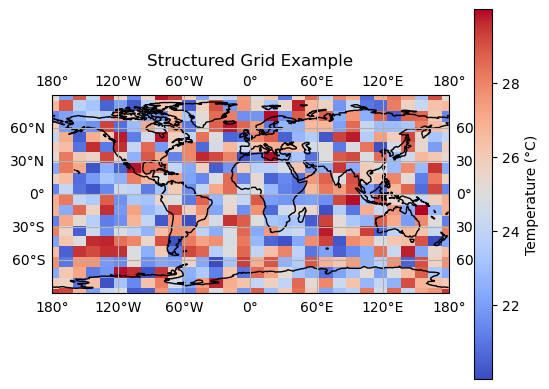
This code below shows a structured mesh example over 2D earth geometry and plots random temperature data.
Given the number of points in longitude and latitude direction, the code uses Numpy’s meshgrid to generates a structured grid. The temperature data is then interpolated onto this grid, creating a smooth representation. Xarray is leveraged to organize the gridded data into a dataset, facilitating easy manipulation and visualization. The resulting plot showcases the data on this structure mesh, providing a clearer understanding of temperature variations across defined longitude and latitude ranges. Plotting the structured grid and the temperature data is done using Cartopy, a cartographic plotting library.
There are many other libraries and ways to create a structured grids.
import cartopy.crs as ccrs
import matplotlib.pyplot as plt
import numpy as np
import xarray as xr

# Define the global domain
lat_range = [-90.0, 90.0]
lon_range = [-180.0, 180.0]

# Create a structured grid. Note the number of points in each dimension
# There is not need to store the grid points in a separate array
# Also note that the grid points are evenly spaced and not connectivity information is needed

num_lat_points = 20
num_lon_points = 30

lats = np.linspace(lat_range[0], lat_range[1], num_lat_points)
lons = np.linspace(lon_range[0], lon_range[1], num_lon_points)

lons_grid, lats_grid = np.meshgrid(lons, lats)

# Generate random temperature data for each grid point
temperature_data = np.random.uniform(
    low=20, high=30, size=(num_lat_points, num_lon_points)
)

# Create xarray Dataset
ds = xr.Dataset()
ds["temperature"] = (["lat", "lon"], temperature_data)
ds["lon"] = lons
ds["lat"] = lats

# Plot the structured grid using xarray
fig, ax = plt.subplots(subplot_kw={"projection": ccrs.PlateCarree()})
ax.set_global()

# Plot world map lines
ax.coastlines()
ax.gridlines(draw_labels=True, dms=True, x_inline=False, y_inline=False)

# Plot the structured grid
cs = ax.pcolormesh(
    ds["lon"], ds["lat"], ds["temperature"], cmap="coolwarm", shading="auto"
)

# Colorbar
cbar = plt.colorbar(cs, ax=ax, label="Temperature (°C)")

ax.set_title("Structured Grid Example")
plt.show()
/home/runner/miniconda3/envs/unstructured-grid-viz-cookbook-dev/lib/python3.10/site-packages/cartopy/io/__init__.py:241: DownloadWarning: Downloading: https://naturalearth.s3.amazonaws.com/110m_physical/ne_110m_coastline.zip
  warnings.warn(f'Downloading: {url}', DownloadWarning)
Unstructured Grids
Characteristic features of unstructured grids are:
Adaptability to complex geometries: Fits intricate shapes and boundaries
Often runs faster than structured grids: Requires fewer elements to achieve similar accuracy
Local refinement: Concentrates resolution on areas of interest
Flexibility in element types: Accommodates various element shapes
Efficient parallelization: Scales well to multiple processors
Suitability for dynamic simulations: Adapts to changing conditions
There are a variety of libraries and conventions for creating unstructured grids. Here we use a very basic standard python approach to showcase an unstructured grid:
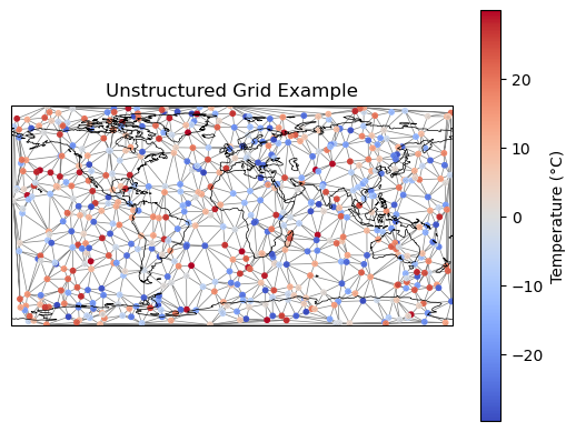
The code generates an unstructured grid over a rectangular domain defined by latitude and longitude ranges. It creates a set of points using matplotlib.tri.Triangulation. The resulting triangulation is then plotted using cartopy and matplotlib.
The are many other types of elements that can be used to create unstructured grids. Polygonal elements are often used to represent complex geometries. Meshes often contain mixed elements with different types of elements used in different areas of the domain.
import cartopy.crs as ccrs
import matplotlib.pyplot as plt
import matplotlib.tri as mtri
import numpy as np
import xarray as xr

# Generate random temperature data
np.random.seed(42)
num_points = 600
latitudes = np.random.uniform(low=-90, high=90, size=num_points)
longitudes = np.random.uniform(low=-180, high=180, size=num_points)
temperatures = np.random.uniform(low=-30, high=30, size=num_points)

# Create xarray DataArray for temperature data
temperature_data = xr.DataArray(
    temperatures, dims="points", coords={"points": range(num_points)}
)

# Perform Delaunay triangulation
triang = mtri.Triangulation(longitudes, latitudes)

# Create xarray DataArray for triangulation coordinates
triang_data = xr.DataArray(
    np.column_stack([triang.x, triang.y]), dims=("points", "coords")
)

# Plot the globe with unstructured mesh using xarray
fig, ax = plt.subplots(subplot_kw={"projection": ccrs.PlateCarree()})
ax.set_global()

# Plot world map lines with prominent gridlines
ax.coastlines(linewidth=0.5)
# ax.gridlines(draw_labels=True, dms=True, x_inline=False, y_inline=False, linewidth=0.5)

# Plot unstructured mesh with bold lines
ax.triplot(
    triang, "ko-", markersize=0.1, linewidth=0.5, alpha=0.5
)  # Increase linewidth to see the triangles

# Scatter plot with temperature data
sc = ax.scatter(
    longitudes,
    latitudes,
    c=temperature_data,
    cmap="coolwarm",
    s=10,
    transform=ccrs.PlateCarree(),
)

# Colorbar
cbar = plt.colorbar(sc, ax=ax, label="Temperature (°C)")

ax.set_title("Unstructured Grid Example")
plt.show()
Note:
This is a very basic example of an unstructured grid with triangles. There are very specialized libraries to create unstructured grids. Often the region of interest is meshed with a finer resolution. The mesh is then coarsened in areas where the resolution is not needed. This is done to reduce the number of elements and improve computational efficiency.
Why UXarray for Unstructured Grids?
UXarray, which stands for “Unstructured-Xarray”, is a Python package that provides Xarray-styled functionality for working with unstructured grids built around the UGRID conventions. UXarray can simplify working with unstructured grids because it:
Enables significant data analysis and visualization functionality to be executed directly on unstructured grids
Adheres to the UGRID specifications for compatibility across a variety of mesh formats
Provides a single interface for supporting a variety of unstructured grid formats including UGRID, MPAS, SCRIP, and Exodus
Inherits from Xarray, providing simplified data using familiar (Xarray-like) data structures and operations
Brings standardization to unstructured mesh support for climate data analysis and visualization
Builds on optimized data structures and algorithms for handling large and complex unstructured datasets
Supports enhanced interoperability and community collaboration
Note:
This notebook serves as an introduction to unstructured grids and UXarray. For more information, please visit the UXarray documentation and specifically see the Usage examples section.
What is next?
The next sections will start with basic building blocks of UXarray and then slowly dive into more advanced features.