Plotting API
UXarray provides a feature-rich plotting API for visualizing unstructured grids, with or without data variables.
This notebook introduces how to interface with the plotting methods through UXarray’s core data structures and provides an introduction to methods that are covered in detail in the next sections.
See also:
This notebook acts as an introduction into using the UXarray plotting API. Please refer to the following notebooks in this chapter for a detailed overview of visualization techniques for different purposes (e.g. Grid Topology, Polygons)
UXarray Plotting API Design
Before jumping into any code, let’s take a look at a high-level snapshot of UXarray’s API design from an Unifed Modeling Language (UML)-like standpoint.
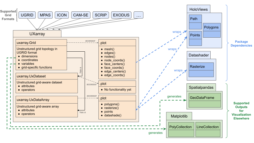
Key takeaways from this design are that:
UXarray’s unified grid representation (through the UGRID conventions) means that all visualization functionality is agnostic to the grid format initially provided by the user.
Each Uxarray data structure (i.e.
Grid,UxDataset,UxDataArray) has its own.plotaccessor, which is used to call plotting routines.The visualization functionality through these
.plotaccessors use HoloViz packages’ plotting functions, wrapping them in a way to exploit all the information that comes from unstructured grids (e.g. connectivity) and provide our unstructured grids-specific functions in the most convenient way for the user.Gridadditionally provides conversion functions that generateSpatialPandas.GeoDataFrameas well asMatplotlib.PolyCollectionandMatplotlib.LineCollectiondata structures to be visualized in HoloViz packages and Matplotlib, respectively, at the user’s own convenience.
Now, we can see the API in action on a sample dataset.
Imports
import uxarray as ux
Data
The grid and data files used in this notebook are from 480km MPAS Ocean model output.
base_path = "../../meshfiles/"
grid_filename = base_path + "oQU480.grid.nc"
data_filename = base_path + "oQU480.data.nc"
grid = ux.open_grid(grid_filename)
grid
<uxarray.Grid>
Original Grid Type: MPAS
Grid Dimensions:
  * n_node: 3947
  * n_edge: 5754
  * n_face: 1791
  * n_max_face_nodes: 6
  * n_max_face_edges: 6
  * n_max_face_faces: 6
  * n_max_node_faces: 3
  * two: 2
  * n_nodes_per_face: (1791,)
Grid Coordinates (Spherical):
  * node_lon: (3947,)
  * node_lat: (3947,)
  * edge_lon: (5754,)
  * edge_lat: (5754,)
  * face_lon: (1791,)
  * face_lat: (1791,)
Grid Coordinates (Cartesian):
  * node_x: (3947,)
  * node_y: (3947,)
  * node_z: (3947,)
  * edge_x: (5754,)
  * edge_y: (5754,)
  * edge_z: (5754,)
  * face_x: (1791,)
  * face_y: (1791,)
  * face_z: (1791,)
Grid Connectivity Variables:
  * face_node_connectivity: (1791, 6)
  * face_edge_connectivity: (1791, 6)
  * face_face_connectivity: (1791, 6)
  * edge_node_connectivity: (5754, 2)
  * edge_face_connectivity: (5754, 2)
  * node_face_connectivity: (3947, 3)
Grid Descriptor Variables:
  * face_areas: (1791,)
  * n_nodes_per_face: (1791,)
  * edge_face_distances: (5754,)
  * edge_node_distances: (5754,)
uxds = ux.open_dataset(grid_filename, data_filename)
uxds
<xarray.UxDataset> Size: 14kB
Dimensions:      (n_face: 1791)
Dimensions without coordinates: n_face
Data variables:
bottomDepth (n_face) float64 14kB ...Grid
Since a Grid instance only contains information about the topology of an unstructured grid (a.k.a. no data variables), the visualizations generated from the Grid class only showcase the coordinates and connectivity.
By default, the Grid.plot method renders the borders of each of the faces.
grid.plot(title="Default Grid Plot")
The UXarray plotting API is written with HoloViews, with the default backend used for generating plots being bokeh. This means that by default, all plots are enabled with interactive features such as panning and zooming. In addition to bokeh, UXarray also supports the matplotlib backend.
For the remainder of this notebook, we will use the matplotlib backend to generate static plots.
grid.plot(
    title="Default Grid Plot with Matplotlib",
    backend="matplotlib",
    aspect=2,
    fig_size=500,
)


WARNING:param.main: fig_size option not found for paths plot with matplotlib; similar options include: []

You can call specific plotting routines through the plot accessor
grid.plot.nodes(title="Grid Node Plot", backend="matplotlib", aspect=2, fig_size=500)
WARNING:param.main: fig_size option not found for points plot with matplotlib; similar options include: []

Since each UxDataset and UxDataArray is always linked to a Grid instance through the uxgrid attribute, all of these grid-specific visualizations are accessible by using that attribute.
uxds.uxgrid.plot(
    title="Grid plot through uxgrid attribute",
    backend="matplotlib",
    aspect=2,
    fig_size=500,
)
WARNING:param.main: fig_size option not found for paths plot with matplotlib; similar options include: []

UxDataArray Plotting
The default plotting method is a great starting point for visualizations. It selects what visualization method to use based on the grid element that the data is mapped to (nodes, edges, faces) and the number of elements in the mesh.
uxds["bottomDepth"].plot(
    title="Default UxDataArray Plot", backend="matplotlib", aspect=2, fig_size=500
)
WARNING:param.main: fig_size option not found for polygons plot with matplotlib; similar options include: []
We can also call other plotting methods through the plot accessor, as was the case with the Grid class.
For example, if we wanted to rasterize the polygons and exclude the ones that cross the antimeridian, it would look something like the following.
uxds["bottomDepth"].plot.polygons(
    exclude_antimeridian=False,
    title="Vector Polygon Plot",
    backend="matplotlib",
    aspect=2,
    fig_size=500,
)
WARNING:param.main: exclude_antimeridian option not found for polygons plot with matplotlib; similar options include: []
WARNING:param.main: fig_size option not found for polygons plot with matplotlib; similar options include: []
UxDataset Plotting
As of the most recent release, UXarray does not support plotting functionality through a ux.UxDataset. For instance, if the following commented out code was executed, it would throw an exception.
# uxds.plot()