3D EOFs - Spectral Analysis for Geophysical Data Cookbook

Overview¶

Empirical Orthogonal Function (EOF) analysis identifies dominant patterns of variability in space-time data. Starting from a synthetic 2D field that evolves in time, we reshape the data into a matrix, compute covariance, extract eigenmodes, and interpret the results as either principal components (temporal analysis) or oscillation modes (spatial analysis).

Mathematical background of EOF / PCA on space-time data
Generate a synthetic surface and a time-varying amplitude
Build and analyze the processing matrix (temporal covariance)
Repeat the analysis using spatial covariance
Compare EOF maps and principal component time series

Prerequisites¶

Concepts	Importance	Notes
2D EOFs	Helpful	Same eigen/covariance workflow in two dimensions
Linear algebra	Necessary	Eigenvalues, eigenvectors, covariance matrices

Time to learn: 35

Imports¶

import os

import matplotlib.pyplot as plt
import numpy as np
import seaborn as sns
from IPython.display import HTML
from matplotlib import animation

sns.set_theme(style="whitegrid", context="notebook", font_scale=1.2)

Mathematical background¶

Space-time data matrix¶

Suppose we observe a field $Z(x, y, t)$ on a regular grid with $n_x \times n_y$ spatial points and $n_t$ time steps. After flattening each snapshot, we arrange the data in a processing matrix $\mathbf{X} \in \mathbb{R}^{m \times n_t}$ , where $m = n_x n_y$ and each column is one time snapshot:

\mathbf{X} = \begin{bmatrix} | & | & & | \\ \mathbf{x}_1 & \mathbf{x}_2 & \cdots & \mathbf{x}_{n_t} \\ | & | & & | \end{bmatrix}

(1)

EOF analysis is equivalent to principal component analysis (PCA) applied to the columns or rows of $\mathbf{X}$ , depending on which covariance matrix we choose.

Covariance matrices¶

Two covariance matrices can be formed from the same data matrix:

\mathbf{C}_{\text{time}} = \mathbf{X}^{\mathsf T}\mathbf{X} \qquad (n_t \times n_t)

(2)

\mathbf{C}_{\text{space}} = \mathbf{X}\mathbf{X}^{\mathsf T} \qquad (m \times m)

(3)

$\mathbf{C}_{\text{time}}$ captures temporal co-variability (each entry compares two time indices across all spatial points).
$\mathbf{C}_{\text{space}}$ captures spatial co-variability (each entry compares two spatial locations across all times).

In practice we diagonalize the smaller matrix for computational efficiency.

Eigenvalue problem¶

Let $\mathbf{C}$ denote either covariance matrix. EOF analysis solves the standard eigenvalue problem:

\mathbf{C}\,\mathbf{v}_k = \lambda_k\,\mathbf{v}_k

(4)

where $\lambda_k$ is the variance explained by mode $k$ and $\mathbf{v}_k$ is the corresponding eigenvector.

The fraction of explained variance for mode $k$ is

p_k = \frac{\lambda_k}{\sum_j \lambda_j}

(5)

The interpretation of $\mathbf{v}_k$ depends on which covariance matrix was used (see the two analysis paths below).

Projections: EOFs and principal components¶

Temporal analysis ( $\mathbf{C} = \mathbf{X}^{\mathsf T}\mathbf{X}$ ):

Eigenvectors $\mathbf{v}_k \in \mathbb{R}^{n_t}$ are principal component time series.
Spatial EOF patterns are obtained by projecting the data onto each eigenvector:

\boldsymbol{\psi}_k = \mathbf{X}\,\mathbf{v}_k \in \mathbb{R}^{m}

(6)

Reshaping $\boldsymbol{\psi}_k$ back to $(n_x, n_y)$ gives an EOF map.

Spatial analysis ( $\mathbf{C} = \mathbf{X}\mathbf{X}^{\mathsf T}$ ):

Eigenvectors $\mathbf{v}_k \in \mathbb{R}^{m}$ are oscillation modes (spatial patterns).
Reshape $\mathbf{v}_k$ directly to obtain EOF maps.
Associated principal component time series are:

a_k(t) = \mathbf{X}^{\mathsf T}\,\mathbf{v}_k \in \mathbb{R}^{n_t}

(7)

The data can be approximated as a sum of outer products of spatial and temporal modes.

Generate synthetic data¶

Define the spatial surface¶

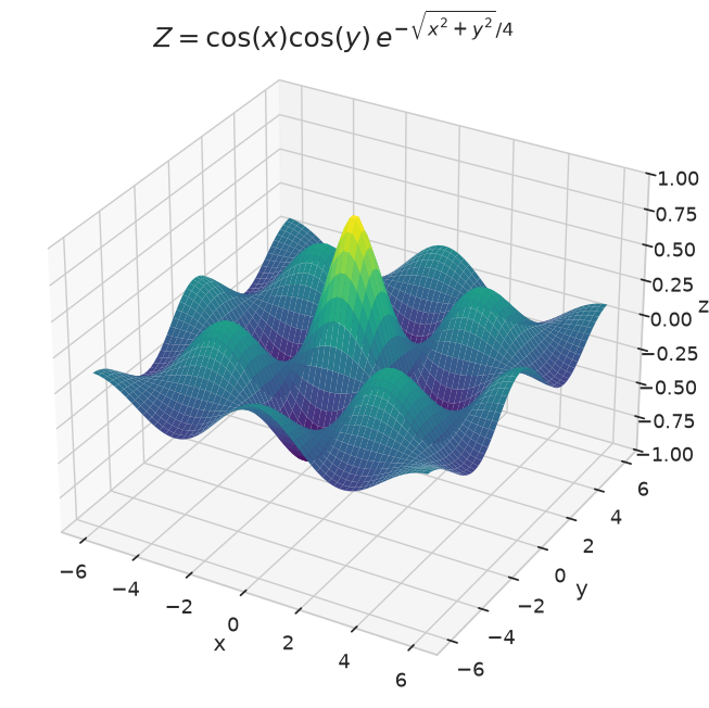
We start with a smooth 2D surface that depends only on $(x, y)$ . This is our basic spatial structure. We choosed to use the following function:

Z = \cos(x) \cos(y) e^{-\sqrt{x^2 + y^2}/4}

(8)

# Function to generate a 2D surface
def surface(x, y):
    return np.cos(x) * np.cos(y) * np.exp(-np.sqrt(x**2 + y**2) / 4)


x = np.linspace(-6, 6, 60)
y = np.linspace(-6, 6, 60)
X, Y = np.meshgrid(x, y)
Z = surface(X, Y)

Z.shape

(60, 60)

Visualize the base surface $Z(x, y)$ before adding any changes in time.

fig = plt.figure(figsize=(8, 8))
plt.suptitle(r"$Z=\cos(x)\cos(y)\,e^{-\sqrt{x^2 + y^2}/4}$", y=0.90, fontsize=18)
ax = plt.axes(projection="3d")
ax.plot_surface(X, Y, Z, rstride=1, cstride=1, cmap="viridis", edgecolor="none")
ax.set_xlabel("x")
ax.set_ylabel("y")
ax.set_zlabel("z")
ax.set_zlim(-1, 1);

Add a time-varying amplitude¶

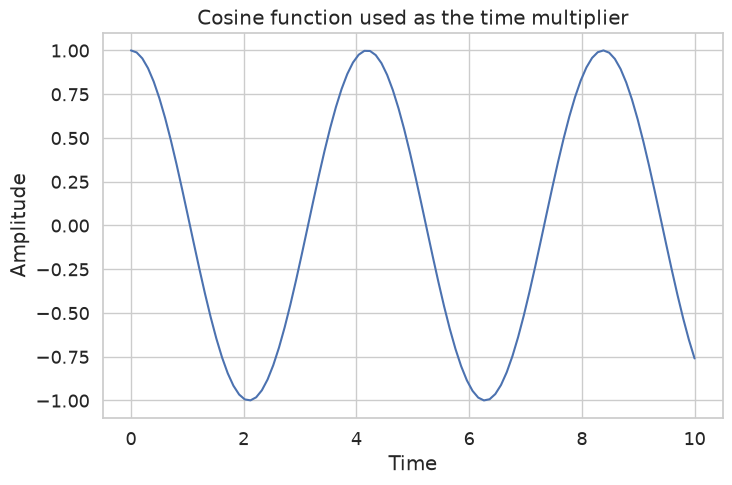
Real geophysical fields rarely stay fixed in time. Here we multiply the surface by a cosine function of time, $\cos(t)$ , to create a simple oscillating amplitude.

time = np.linspace(0, 10, 100)
time_multiplier = np.cos(time*1.5)

fig = plt.figure(figsize=(8, 5))
plt.title("Cosine function used as the time multiplier")
plt.plot(time, time_multiplier)
plt.xlabel("Time")
plt.ylabel("Amplitude");

Introduce a spatial shift over time¶

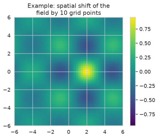
To make the patterns more interesting, each snapshot is also shifted horizontally by an amount that grows with time. The preview below shows a single snapshot shifted by 10 grid points.

shift_amount = 10

plt.title(f"Example: spatial shift of the\nfield by {shift_amount} grid points")
plt.imshow(
    np.roll(Z, shift_amount, axis=1),
    cmap="viridis",
    interpolation="none",
    vmin=-np.max(np.abs(Z)),
    vmax=np.max(np.abs(Z)),
    origin="lower",
    extent=[np.min(X), np.max(X), np.min(Y), np.max(Y)],
)
plt.colorbar()
plt.show()

Build the processing matrix¶

We now construct the space-time data and reshape it into the matrix $\mathbf{X}$ introduced above.

For each time index $t$ :

Z_t(x, y) = Z(x, y)\,\cos(t) \quad \text{and then shifted along } x

(9)

The 3D-data has shape $(n_x, n_y, n_t)$ . Flattening the first two dimensions gives $\mathbf{X}$ with shape $(m, n_t)$ .

data_cube = np.zeros([Z.shape[0], Z.shape[1], len(time_multiplier)])
data_cube.shape

(60, 60, 100)

# Loop over the time indices to create the 3D-data
for time_index, multiplier in enumerate(time_multiplier):
    snapshot = Z * time_multiplier[time_index]
    data_cube[:, :, time_index] = np.roll(snapshot, time_index * 2, axis=1)

print("Data cube shape:", np.shape(data_cube))

Data cube shape: (60, 60, 100)

Animate the space-time field¶

The animation below steps through each snapshot $Z_t(x, y)$ as a 3D surface, showing how the amplitude modulation and horizontal shift evolve together over time.

fig = plt.figure(figsize=(6, 6))
fig.suptitle(r"$Z=\cos(x)\cos(y)\,e^{-\sqrt{x^2 + y^2}/4}$", y=0.98, fontsize=18)
ax = fig.add_subplot(111, projection="3d")


def draw_snapshot(frame):
    ax.clear()
    ax.plot_surface(
        X,
        Y,
        data_cube[:, :, frame],
        rstride=1,
        cstride=1,
        cmap="viridis",
        edgecolor="none",
        vmax=1,
        vmin=-1,
    )
    ax.set_xlabel("x")
    ax.set_ylabel("y")
    ax.set_zlabel("z")
    ax.set_zlim(-1, 1)
    ax.set_title(
        f"t = {time[frame]:.2f}"
    )
    return (ax,)


def init():
    return draw_snapshot(0)


def animate(frame):
    return draw_snapshot(frame)


anim = animation.FuncAnimation(
    fig,
    animate,
    init_func=init,
    frames=len(time),
    interval=50,
    blit=False,
    repeat=True,
)
plt.tight_layout()
plt.close()

HTML(anim.to_jshtml())

data_matrix = data_cube.reshape(
    data_cube.shape[0] * data_cube.shape[1], data_cube.shape[2]
)
print("Processing matrix shape (m x n_t):", np.shape(data_matrix))

Processing matrix shape (m x n_t): (3600, 100)

Part I: Temporal analysis¶

We first analyze $\mathbf{C}_{\text{time}} = \mathbf{X}^{\mathsf T}\mathbf{X}$ , which has shape $(n_t \times n_t)$ . This is the smaller matrix when $n_t \ll m$ .

The eigenvectors of $\mathbf{C}_{\text{time}}$ are principal component time series.

Compute the covariance matrices¶

cov_matrix_1 = data_matrix.T @ data_matrix
cov_matrix_2 = data_matrix @ data_matrix.T

print("C_time = X.T @ X shape:", np.shape(cov_matrix_1))
print("C_space = X @ X.T shape:", np.shape(cov_matrix_2))

C_time = X.T @ X shape: (100, 100)
C_space = X @ X.T shape: (3600, 3600)

We choose the smaller matrix to compute the eigenvalues and eigenvectors. As it is more efficient to compute the eigenvalues and eigenvectors of a smaller matrix.

Eigen-decomposition¶

Solve $\mathbf{C}_{\text{time}}\,\mathbf{v}_k = \lambda_k\,\mathbf{v}_k$ using numpy.linalg.eig. We set analysis_index = 1 to label the results as a temporal analysis.

cov_matrix = cov_matrix_1
eigen_val, eigen_vect = np.linalg.eig(cov_matrix)

analysis_types = ["spatial", "temporal"]
analysis_index = 1  # temporal analysis
eigenvector_roles = ["Oscillation modes", "Principal components"]

Explained variance¶

Each eigenvalue $\lambda_k$ measures how much variance mode $k$ explains. We convert these to percentages using $p_k = 100\,\lambda_k / \sum_j \lambda_j$ .

total_variance = np.sum(eigen_val)
explained_variance_pct = (eigen_val / total_variance) * 100

print("Number of eigenvalues:", np.shape(eigen_val))
print(f"The eigenvectors are the {eigenvector_roles[analysis_index]}")
print("Eigenvector matrix shape:", np.shape(eigen_vect))

Number of eigenvalues: (100,)
The eigenvectors are the Principal components
Eigenvector matrix shape: (100, 100)

fig = plt.figure("Explained variance", facecolor="w", edgecolor="w")
ax = fig.add_subplot(111)
ax.set_title(
    f"Explained variance\nby the {eigenvector_roles[analysis_index]}",
    fontsize=15,
)
ax.plot(np.arange(1, 6), explained_variance_pct[0:5], "k", lw=3)
plt.xlim(1, 5)
ax.set_xlabel("Mode index $k$")
ax.set_ylabel("Explained variance [%]")
plt.xticks(np.arange(1, 6))
plt.grid(True)

/home/runner/micromamba/envs/cookbook-dev/lib/python3.14/site-packages/matplotlib/cbook.py:1810: ComplexWarning: Casting complex values to real discards the imaginary part
  return math.isfinite(val)
/home/runner/micromamba/envs/cookbook-dev/lib/python3.14/site-packages/matplotlib/cbook.py:1407: ComplexWarning: Casting complex values to real discards the imaginary part
  return np.asanyarray(x, float)

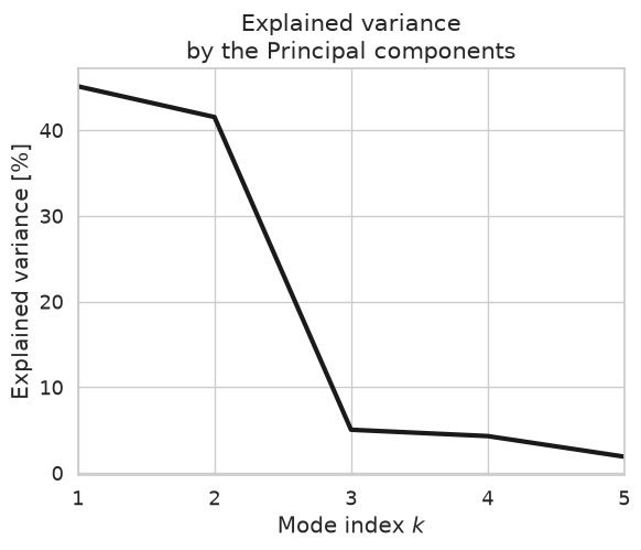
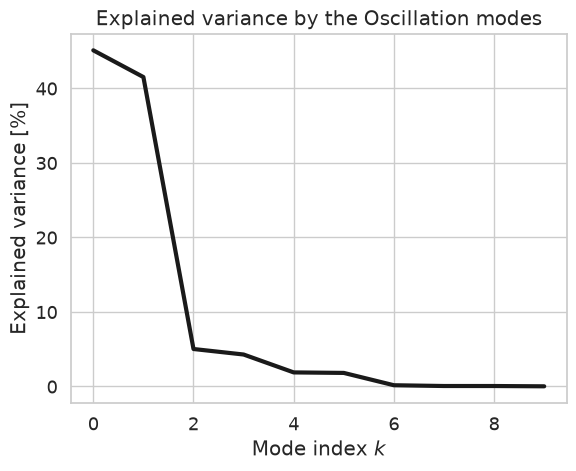
The previous plot shows the explained variance of the first 5 modes, where first couple of modes explain most of the variance of the data.

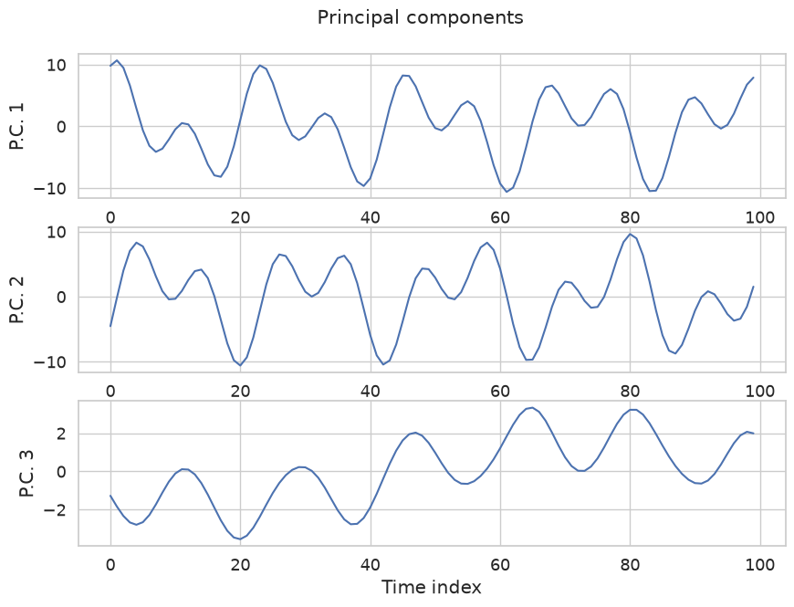
Inspect the leading eigenvectors¶

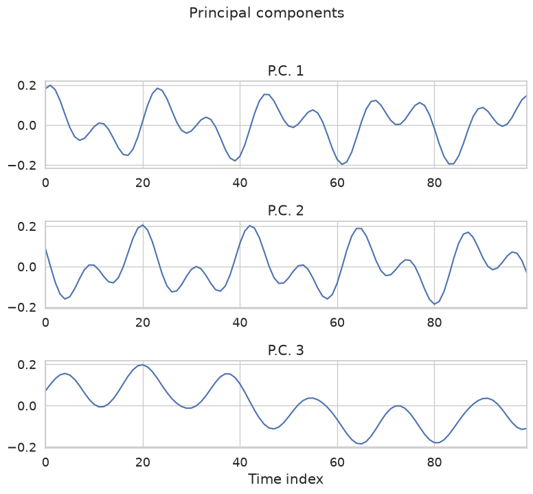
Plot the first three eigenvectors $\mathbf{v}_1, \mathbf{v}_2, \mathbf{v}_3$ . Because we used $\mathbf{C}_{\text{time}}$ , each curve is a principal component time series of length $n_t$ .

Always inspect eigenvectors visually to confirm they are physically meaningful.

eigen_vect_1 = eigen_vect[:, 0]
eigen_vect_2 = eigen_vect[:, 1]
eigen_vect_3 = eigen_vect[:, 2]

plot_labels = ["O.M.", "P.C."]

fig = plt.figure(edgecolor="w", figsize=(8, 7))
plt.suptitle(f"{eigenvector_roles[analysis_index]}", y=1.03, fontsize=15)

for mode_index, mode in enumerate([eigen_vect_1, eigen_vect_2, eigen_vect_3], start=1):
    ax = fig.add_subplot(3, 1, mode_index)
    plt.title(f"{plot_labels[analysis_index]} {mode_index}")
    ax.plot(mode)
    plt.grid(True)
    plt.xlim(0, len(time) - 1)

plt.xlabel("Time index")
plt.tight_layout()

Principal components should be uncorrelated at zero lag. The lagged cross-correlation below checks whether pairs of leading modes remain independent at different time offsets.

plt.figure(figsize=(12, 4))
plt.suptitle("Lagged correlation between principal components", y=1.05, fontsize=18)

pairs = [
    ("A. P.C. 1 and P.C. 2", eigen_vect[:, 0], eigen_vect[:, 1]),
    ("B. P.C. 1 and P.C. 3", eigen_vect[:, 0], eigen_vect[:, 2]),
    ("C. P.C. 2 and P.C. 3", eigen_vect[:, 1], eigen_vect[:, 2]),
]

for subplot_index, (title, mode_a, mode_b) in enumerate(pairs, start=1):
    plt.subplot(1, 3, subplot_index)
    plt.title(title, fontsize=15, loc="right")
    plt.xcorr(mode_a, mode_b, maxlags=50, lw=2)
    if subplot_index == 1:
        plt.ylabel("Correlation coefficient")
    plt.xlabel("Lag")
    plt.ylim(-1, 1)
    plt.xlim(0, 30)

plt.tight_layout()

/home/runner/micromamba/envs/cookbook-dev/lib/python3.14/site-packages/numpy/ma/core.py:3452: ComplexWarning: Casting complex values to real discards the imaginary part
  _data[indx] = dval

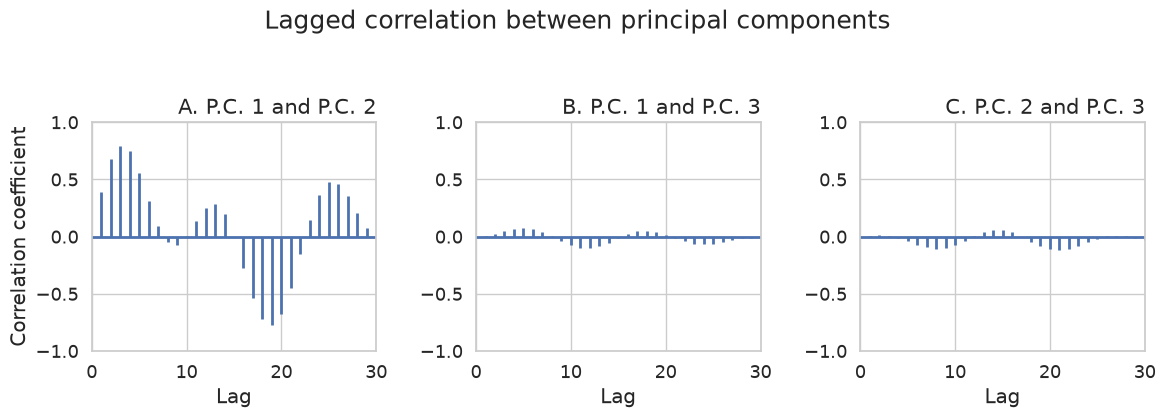
Here, we can see that the first two principal components are uncorrelated at zero lag but exhibit a significant correlation at a lag of around 12 time steps. This is representative of the propagation pattern captured by the first 2 components, which is due to how the data was built.

In real geophysical datasets, propagating signals are also frequently represented by pairs of consecutive modes with similar explained variance. Such mode pairs often correspond to oscillatory or traveling phenomena, with the phase information distributed between the two principal components.

Project onto eigenvectors to obtain EOF maps¶

Spatial EOF patterns follow from the projection $\boldsymbol{\psi}_k = \mathbf{X}\,\mathbf{v}_k$ . Each $\boldsymbol{\psi}_k$ is a vector of length $m$ (one value per grid point).

print(
    "Projection dimensions:\n"
    f"  data_matrix: {data_matrix.shape}\n"
    f"  eigenvector: {eigen_vect[:, 0].shape}"
)

Projection dimensions:
  data_matrix: (3600, 100)
  eigenvector: (100,)

eof_1 = data_matrix @ eigen_vect[:, 0]
eof_2 = data_matrix @ eigen_vect[:, 1]
eof_3 = data_matrix @ eigen_vect[:, 2]

print("EOF vector length (number of spatial points):", eof_1.shape)

EOF vector length (number of spatial points): (3600,)

Reshape each EOF vector $\boldsymbol{\psi}_k$ from length $m$ back to the original grid shape $(n_x, n_y)$ so it can be displayed as a map.

eof_1 = eof_1.reshape(data_cube.shape[0], data_cube.shape[1])
eof_2 = eof_2.reshape(data_cube.shape[0], data_cube.shape[1])
eof_3 = eof_3.reshape(data_cube.shape[0], data_cube.shape[1])

print("EOF map shape:", eof_1.shape)

EOF map shape: (60, 60)

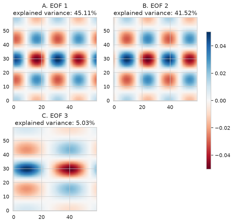
The three leading EOF maps below are colored by amplitude. The subtitle on each panel shows the explained variance fraction $p_k$ from the temporal eigenvalues.

fig = plt.figure(figsize=(8, 8))
eof_maps = [eof_1, eof_2, eof_3]
panel_labels = ["A", "B", "C"]

for index, (eof_map, label) in enumerate(zip(eof_maps, panel_labels), start=1):
    plt.subplot(2, 2, index)
    vmax = np.max(np.abs(eof_map.astype(float)))
    im = plt.imshow(
        eof_map.astype(float),
        interpolation="none",
        vmin=-vmax,
        vmax=vmax,
        origin="lower",
        cmap="RdBu",
    )
    if index == 1:
        color_mappable = im
    plt.title(
        f"{label}. EOF {index}\n"
        f"explained variance: {np.real(explained_variance_pct[index - 1]):.2f}%",
        fontsize=15,
    )

plt.subplots_adjust(bottom=0, right=0.93)
cbaxes = fig.add_axes([0.97, 0.2, 0.02, 0.6])
plt.colorbar(color_mappable, cax=cbaxes)

/tmp/ipykernel_4083/1158140069.py:7: ComplexWarning: Casting complex values to real discards the imaginary part
  vmax = np.max(np.abs(eof_map.astype(float)))
/tmp/ipykernel_4083/1158140069.py:9: ComplexWarning: Casting complex values to real discards the imaginary part
  eof_map.astype(float),

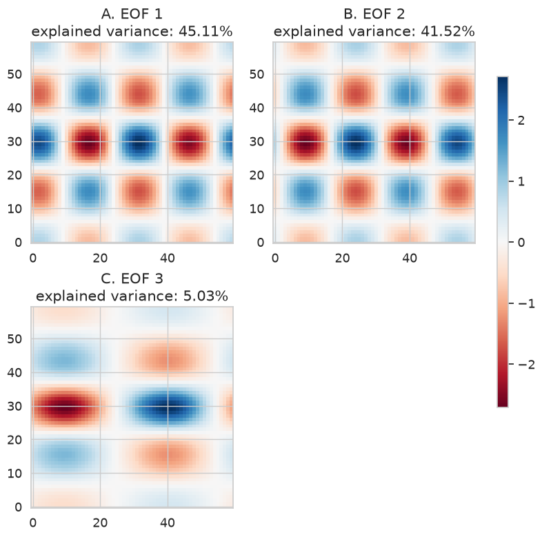
The first two EOFs have nearly identical spatial structure, differing mainly by a horizontal translation. Together they form a propagating mode pair: the phase information is split across the two patterns, while their associated principal components capture the $\cos(t)$ amplitude modulation as the field shifts in time. The third EOF isolates the spatial translation itself, the cumulative horizontal shift applied at each time step.

Part II: Spatial analysis¶

Now we switch to the other covariance matrix:

\mathbf{C}_{\text{space}} = \mathbf{X}\mathbf{X}^{\mathsf T}

(10)

This matrix has shape $(m \times m)$ . Its eigenvectors $\mathbf{v}_k \in \mathbb{R}^{m}$ are oscillation modes: spatial patterns that co-vary across time. The associated principal component time series are $a_k = \mathbf{X}^{\mathsf T}\mathbf{v}_k$ .

Recompute covariance and eigenmodes¶

cov_matrix_1 = data_matrix.T @ data_matrix
cov_matrix_2 = data_matrix @ data_matrix.T

print("C_time shape:", np.shape(cov_matrix_1))
print("C_space shape:", np.shape(cov_matrix_2))

C_time shape: (100, 100)
C_space shape: (3600, 3600)

We are going to user the larger matrix to compute the eigenvalues and eigenvectors.

cov_matrix = cov_matrix_2
eigen_val, eigen_vect = np.linalg.eig(cov_matrix)

analysis_index = 0  # spatial analysis

Explained variance and leading spatial modes¶

The explained variance fractions use the same formula $p_k = 100\,\lambda_k / \sum_j \lambda_j$ , but now $\lambda_k$ comes from $\mathbf{C}_{\text{space}}$ .

total_variance = np.sum(eigen_val)
explained_variance_pct = (eigen_val / total_variance) * 100

print("Number of eigenvalues:", np.shape(eigen_val))
print(f"The eigenvectors are the {eigenvector_roles[analysis_index]}")
print("Eigenvector matrix shape:", np.shape(eigen_vect))

Number of eigenvalues: (3600,)
The eigenvectors are the Oscillation modes
Eigenvector matrix shape: (3600, 3600)

fig = plt.figure("Explained variance", facecolor="w", edgecolor="w")
ax = fig.add_subplot(111)
ax.set_title(f"Explained variance by the {eigenvector_roles[analysis_index]}")
ax.plot(explained_variance_pct[0:10], "k", lw=3)
ax.set_xlabel("Mode index $k$")
ax.set_ylabel("Explained variance [%]")
plt.grid(True)

Each eigenvector is now a spatial mode. Plot the first three entries as a function of spatial index before reshaping them into maps.

eigen_vect_1 = eigen_vect[:, 0]
eigen_vect_2 = eigen_vect[:, 1]
eigen_vect_3 = eigen_vect[:, 2]

EOF maps from spatial eigenvectors¶

When $\mathbf{C} = \mathbf{X}\mathbf{X}^{\mathsf T}$ , the eigenvectors are the spatial EOF patterns. Reshape each $\mathbf{v}_k$ directly—no matrix multiplication needed:

\text{EOF map}_k = \text{reshape}(\mathbf{v}_k) \in \mathbb{R}^{n_x \times n_y}

(11)

eof_1 = eigen_vect_1.reshape(data_cube.shape[0], data_cube.shape[1])
eof_2 = eigen_vect_2.reshape(data_cube.shape[0], data_cube.shape[1])
eof_3 = eigen_vect_3.reshape(data_cube.shape[0], data_cube.shape[1])

fig = plt.figure(figsize=(8, 8))
eof_maps = [eof_1, eof_2, eof_3]
panel_labels = ["A", "B", "C"]

for index, (eof_map, label) in enumerate(zip(eof_maps, panel_labels), start=1):
    plt.subplot(2, 2, index)
    vmax = np.max(np.abs(eof_map.astype(float)))
    im = plt.imshow(
        eof_map.astype(float),
        interpolation="none",
        vmin=-vmax,
        vmax=vmax,
        origin="lower",
        cmap="RdBu",
    )
    if index == 1:
        color_mappable = im
    plt.title(
        f"{label}. EOF {index}\n"
        f"explained variance: {np.real(explained_variance_pct[index - 1]):.2f}%",
        fontsize=15,
    )

plt.subplots_adjust(bottom=0, right=0.93)
cbaxes = fig.add_axes([0.97, 0.2, 0.02, 0.6])
plt.colorbar(color_mappable, cax=cbaxes)

/tmp/ipykernel_4083/1158140069.py:7: ComplexWarning: Casting complex values to real discards the imaginary part
  vmax = np.max(np.abs(eof_map.astype(float)))
/tmp/ipykernel_4083/1158140069.py:9: ComplexWarning: Casting complex values to real discards the imaginary part
  eof_map.astype(float),

Principal component time series¶

Project the data onto the spatial eigenvectors to recover the time evolution of each mode:

a_k = \mathbf{X}^{\mathsf T}\,\mathbf{v}_k

(12)

Each $a_k$ is a principal component time series of length $n_t$ .

print(
    "Projection dimensions:\n"
    f"  data_matrix.T: {data_matrix.T.shape}\n"
    f"  eigenvector: {eigen_vect[:, 0].shape}"
)

Projection dimensions:
  data_matrix.T: (100, 3600)
  eigenvector: (3600,)

principal_component_1 = data_matrix.T @ eigen_vect[:, 0]
principal_component_2 = data_matrix.T @ eigen_vect[:, 1]
principal_component_3 = data_matrix.T @ eigen_vect[:, 2]

print("Principal component length (number of time steps):", principal_component_3.shape)

Principal component length (number of time steps): (100,)

analysis_index = 1
plot_labels = ["O.M.", "P.C."]

fig = plt.figure(edgecolor="w", figsize=(10, 7))
plt.suptitle(f"{eigenvector_roles[analysis_index]}", y=0.95, fontsize=15)

for mode_index, component in enumerate(
    [principal_component_1, principal_component_2, principal_component_3], start=1
):
    ax = fig.add_subplot(3, 1, mode_index)
    ax.set_ylabel(f"{plot_labels[analysis_index]} {mode_index}")
    ax.plot(component)
    plt.grid(True)
    ax.set_xlabel("Time index")

Summary¶

We applied EOF analysis to a synthetic space-time field. The key steps were:

Arrange snapshots in a processing matrix $\mathbf{X}$ .
Form either $\mathbf{C}_{\text{time}} = \mathbf{X}^{\mathsf T}\mathbf{X}$ or $\mathbf{C}_{\text{space}} = \mathbf{X}\mathbf{X}^{\mathsf T}$ .
Solve $\mathbf{C}\,\mathbf{v}_k = \lambda_k\,\mathbf{v}_k$ and rank modes by explained variance $p_k$ .
Interpret eigenvectors as temporal PCs or spatial modes, then project to obtain the complementary EOF maps or PC time series.

The choice of covariance matrix determines which patterns are extracted directly as eigenvectors and which must be computed by projection.

What’s next?¶

TBD