Harmonic Analysis of the Seasonal Cycle

Overview¶

The seasonal cycle is the most prominent mode of variability in many climate variables. In this notebook we use harmonic analysis, representing a time series as a sum of sine and cosine waves, to describe the monthly climatology of sea surface temperature (SST) at a single location, closely following Section 10.4 of Wilks (2019)

We will:

Load NOAA Optimum Interpolation SST V2 daily data and build a monthly climatology.
Approximate the climatology with a single cosine wave using an “eyeballed” amplitude and phase.
Estimate the amplitude and phase of the first harmonic by least squares using the analysis equations (Wilks (2019) Eqs. 10.60 and 10.59).
Extend the analysis to higher harmonics and quantify how much of the variance each harmonic explains.
Reconstruct the climatology exactly using all n/2 harmonics.
Use the phase-shift trick of Wilks Ex. 10.10 to evaluate the fitted cosine on a daily time axis.

Prerequisites¶

Concepts	Importance	Notes

Time to learn: ~---- minutes.

Imports¶

All packages used in the rest of the notebook are imported up front. s3fs is configured to read anonymously from the public Pythia bucket on the Jetstream2 S3 endpoint.

import numpy as np
import pandas as pd
import matplotlib.pyplot as plt
import seaborn as sns

import s3fs
import xarray as xr

sns.set_theme(style="whitegrid", context="notebook", font_scale=1.2)

URL = "https://js2.jetstream-cloud.org:8001/"
fs = s3fs.S3FileSystem(anon=True, client_kwargs=dict(endpoint_url=URL))

The data: NOAA OI SST V2¶

We use the daily, 2.5°-regridded NOAA Optimum Interpolation SST V2 Reynolds et al., 2007 avialable on the Pythia Jetstream2 S3 bucket as a Zarr store. The full record runs from September 1981 to the present and covers the tropics from 30°S to 30°N. The cell below opens the store lazily, no data are actually transferred until we compute something.

sst_noaa_oi_store = s3fs.S3Map(
    root="pythia/sst_noaa_oi.zarr",
    s3=fs,
    check=False,
)

sst_noaa_oi = xr.open_zarr(sst_noaa_oi_store)

if "__xarray_dataarray_variable__" in sst_noaa_oi.data_vars:
    sst_noaa_oi = sst_noaa_oi.rename_vars(
        {"__xarray_dataarray_variable__": "sst"}
    )

sst_noaa_oi

From daily to monthly¶

We first restrict the record to complete calendar years (1982–2025) and aggregate the daily field to monthly means using xarray.Dataset.resample. We then pick a single grid point — lat=0°, lon=200°E (central equatorial Pacific), and look at its seasonal cycle.

year_initial = 1982
year_final = 2025

sst_noaa_oi = sst_noaa_oi.sel(
    time=slice(f"{year_initial}-01-01", f"{year_final}-12-31")
)

sst_noaa_oi_monthly = sst_noaa_oi.resample(time="MS").mean()

lat_select = 0.0
lon_select = 200.0

sst_series = sst_noaa_oi_monthly["sst"].sel(
    lat=lat_select, lon=lon_select, method="nearest"
)

time_value = pd.to_datetime(sst_noaa_oi_monthly.time[0].values)

fig, ax = plt.subplots(figsize=(8, 4))
sst_noaa_oi_monthly["sst"][0].plot(ax=ax)
ax.plot(lon_select, lat_select, "ro", markersize=10)
ax.set_title(
    f"Selected location (lat={lat_select}, lon={lon_select})\n"
    f"background: monthly mean SST on {time_value:%Y-%m}"
)
ax.set_xlabel("Longitude")
ax.set_ylabel("Latitude")
plt.show()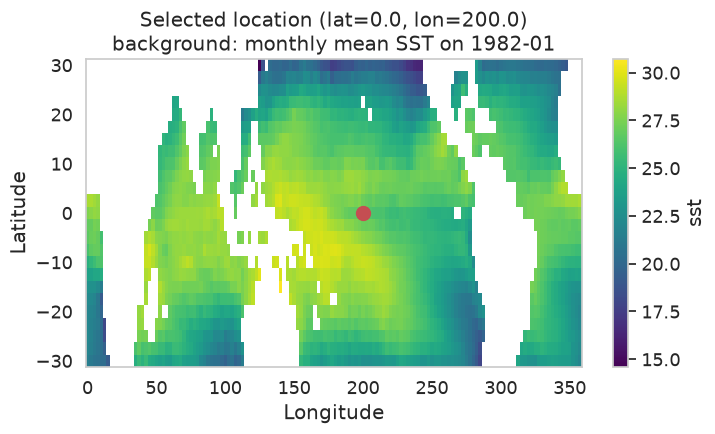

fig, ax = plt.subplots(figsize=(8, 4))
sst_series.plot(ax=ax)
ax.set_title(
    f"Monthly SST at (lat={lat_select}, lon={lon_select})  "
    f"{year_initial}–{year_final}"
)
ax.set_xlabel("Time")
ax.set_ylabel("SST (°C)")
plt.show()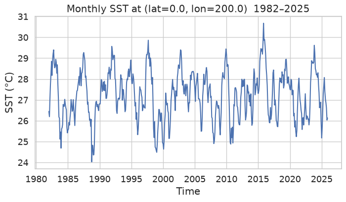

The monthly climatology¶

We average all Januaries together, all Februaries, etc., to obtain a 12-month climatology $\{y_t,\; t=1,\dots,12\}$ . This is the “data series” that the rest of the notebook will try to model.

sst_monthly_climatology = sst_series.groupby("time.month").mean("time")

fig, ax = plt.subplots(figsize=(8, 4))
sst_monthly_climatology.plot(ax=ax, marker="o")
ax.set_title(
    f"Monthly climatology of SST  (lat={lat_select}, lon={lon_select})"
)
ax.set_xlabel("Month, $t$")
ax.set_ylabel("SST (°C)")
ax.set_xticks(np.arange(1, 13))
plt.show()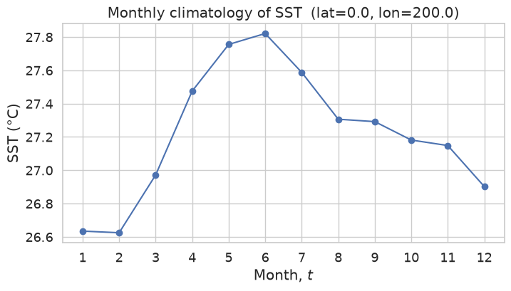

A single cosine wave¶

A simple harmonic representation of a series of length $n$ is:

y_t \;=\; \bar{y} \,+\, C_1 \cos\!\left(\frac{2\pi t}{n} - \phi_1\right), \qquad t = 1, 2, \dots, n,

(1)

with three parameters: the mean $\bar{y}$ , the amplitude $C_1$ , and the phase $\phi_1$ . The cosine is preferred over the sine because $\phi_1$ then has the clean interpretation “angle of the maximum”, so the function peaks at $t = \phi_1\, n / 2\pi$ .

As a first guess we set:

$\bar{y}$ = sample mean of the climatology,
$C_1$ = half the peak-to-peak range, and
$\phi_1$ corresponds to the month containing the warmest mean SST.

y = sst_monthly_climatology.values
t = sst_monthly_climatology["month"].values.astype(float)
n = len(y)
y_mean = float(np.mean(y))

print(f"n         = {n}   (samples per year)")
print(f"mean SST  = {y_mean:.3f} °C")
print(f"range     = {y.min():.3f} … {y.max():.3f} °C")

n         = 12   (samples per year)
mean SST  = 27.225 °C
range     = 26.625 … 27.821 °C

amp_eyeball = (y.max() - y.min()) / 2.0
peak_month = int(t[np.argmax(y)])
phase_eyeball = 2.0 * np.pi * peak_month / n

print(f"Eyeballed amplitude C1  ≈ {amp_eyeball:.3f} °C")
print(f"Peak month (argmax)     = {peak_month}")
print(f"Eyeballed phase   φ1    ≈ {np.degrees(phase_eyeball):.1f}°")

cosine_fit_eyeball = (
    y_mean + amp_eyeball * np.cos(2 * np.pi * t / n - phase_eyeball)
)

Eyeballed amplitude C1  ≈ 0.598 °C
Peak month (argmax)     = 6
Eyeballed phase   φ1    ≈ 180.0°

fig, ax = plt.subplots(figsize=(9, 4))
ax.plot(t, y, "o", label="Monthly climatology")
ax.plot(t, cosine_fit_eyeball, "r--", label="Eyeballed Cosine Fit")
ax.axhline(y_mean, color="0.6", lw=0.8, label="Mean $\\bar{y}$")
ax.set_title("Single-harmonic fit by inspection")
ax.set_xlabel("Month, $t$")
ax.set_ylabel("SST (°C)")
ax.set_xticks(np.arange(1, 13))
ax.legend(loc="upper right", fontsize=10)
plt.show()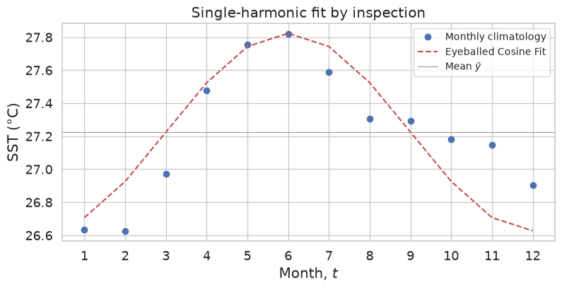

As we see, the eyeballed cosine fit is not a good fit for the data. We will now use least squares to fit the first harmonic to the data.

Least-squares first harmonic¶

Using the trigonometric identity:

\cos(\alpha-\phi) = \cos\phi\cos\alpha + \sin\phi\sin\alpha

(2)

We can rewrite the equation of the previous section as a linear combination of an unshifted cosine and an unshifted sine:

y_t \;=\; \bar{y} \,+\, A_1 \cos\!\left(\tfrac{2\pi t}{n}\right) \,+\, B_1 \sin\!\left(\tfrac{2\pi t}{n}\right), \qquad \begin{aligned} A_1 &= C_1 \cos\phi_1, \\ B_1 &= C_1 \sin\phi_1. \end{aligned}

(3)

In this form $A_1$ and $B_1$ are ordinary regression slopes, they could be obtained by feeding $\cos(2\pi t/n)$ and $\sin(2\pi t/n)$ as predictors into any linear regression model.

For data that are evenly spaced with no missing values (our case), the least-squares estimates collapse to the “analysis equations”:

A_1 = \frac{2}{n}\sum_{t=1}^{n} y_t \cos\!\left(\tfrac{2\pi t}{n}\right), \qquad B_1 = \frac{2}{n}\sum_{t=1}^{n} y_t \sin\!\left(\tfrac{2\pi t}{n}\right),

(4)

and the amplitude/phase:

C_1 = \sqrt{A_1^2 + B_1^2}, \qquad \phi_1 = \operatorname{atan2}(B_1,\, A_1).

(5)

omega_t = 2.0 * np.pi * t / n

A1 = (2.0 / n) * np.sum(y * np.cos(omega_t))
B1 = (2.0 / n) * np.sum(y * np.sin(omega_t))

C1 = np.hypot(A1, B1)
phi1 = np.arctan2(B1, A1) % (2 * np.pi)

print(f"A1   = {A1:8.4f}")
print(f"B1   = {B1:8.4f}")
print(f"C1   = {C1:8.4f}  (least-squares amplitude)")
print(f"phi1 = {np.degrees(phi1):6.2f}°  "
      f"(peak month ≈ {phi1 * n / (2 * np.pi):.2f})")

A1   =  -0.4596
B1   =  -0.1382
C1   =   0.4799  (least-squares amplitude)
phi1 = 196.73°  (peak month ≈ 6.56)

t_fine = np.linspace(1, n, 400)
fit_ls = y_mean + A1 * np.cos(2 * np.pi * t_fine / n) \
                + B1 * np.sin(2 * np.pi * t_fine / n)
fit_eye_fine = y_mean + amp_eyeball * np.cos(
    2 * np.pi * t_fine / n - phase_eyeball
)

fig, ax = plt.subplots(figsize=(8, 4))
ax.plot(t, y, "ko", label="Monthly climatology")
ax.plot(t_fine, fit_eye_fine, "r--", label="Eyeballed Cosine Fit")
ax.plot(t_fine, fit_ls, "b-", label="Least squares")
ax.axhline(y_mean, color="0.6", lw=0.8, label="Mean $\\bar{y}$")
ax.set_title("Comparison: eyeballed vs least-squares first harmonic")
ax.set_xlabel("Month, $t$")
ax.set_ylabel("SST (°C)")
ax.set_xticks(np.arange(1, 13))
ax.legend(loc="upper right", fontsize=10)
plt.show()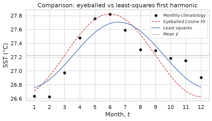

Higher harmonics¶

Just as adding more predictors to a multiple regression always improves the fit, adding more cosine waves of higher frequency always improves the fit of a harmonic representation. Any series of length $n$ can be reproduced exactly by the following equation:

y_t \;=\; \bar{y} \,+\, \sum_{k=1}^{n/2} \left[\, A_k \cos\!\left(\tfrac{2\pi k t}{n}\right) + B_k \sin\!\left(\tfrac{2\pi k t}{n}\right) \right].

(6)

The $k$ -th harmonic completes exactly $k$ full cycles over the $n$ samples; its angular frequency is $\omega_k = 2\pi k/n$ . For evenly spaced data the coefficients are given by the generalized analysis equations:

A_k = \frac{2}{n}\sum_{t=1}^{n} y_t \cos\!\left(\tfrac{2\pi k t}{n}\right), \qquad B_k = \frac{2}{n}\sum_{t=1}^{n} y_t \sin\!\left(\tfrac{2\pi k t}{n}\right),

(7)

with amplitude $C_k = \sqrt{A_k^2 + B_k^2}$ and phase $\phi_k = \operatorname{atan2}(B_k, A_k)$ .

For our monthly climatology $n=12$ , so we can fit up to $n/2 = 6$ harmonics. Because $n$ is even, the phase of the highest harmonic ( $k=n/2$ ) is forced to zero.

Below we build a small helper that returns $(A_k, B_k, C_k, \phi_k)$ for any $k$ , then plot the first three harmonics separately.

def harmonic_coeffs(y, k):
    """
    Return (A_k, B_k, C_k, phi_k) for harmonic k of an evenly-spaced series.

    Implements Wilks Eqs. 10.64 (A_k, B_k) and 10.65 (C_k, phi_k).
    """
    n = len(y)
    t = np.arange(1, n + 1, dtype=float)
    omega_kt = 2.0 * np.pi * k * t / n
    A = (2.0 / n) * np.sum(y * np.cos(omega_kt))
    B = (2.0 / n) * np.sum(y * np.sin(omega_kt))
    C = np.hypot(A, B)
    phi = np.arctan2(B, A) % (2 * np.pi)
    return A, B, C, phi


coeffs = {k: harmonic_coeffs(y, k) for k in range(1, n // 2 + 1)}

print(f"{'k':>2}  {'A_k':>8}  {'B_k':>8}  {'C_k':>8}  {'phi_k (deg)':>12}")
print("-" * 46)
for k, (A, B, C, phi) in coeffs.items():
    print(f"{k:2d}  {A:8.4f}  {B:8.4f}  {C:8.4f}  {np.degrees(phi):12.2f}")

 k       A_k       B_k       C_k   phi_k (deg)
----------------------------------------------
 1   -0.4596   -0.1382    0.4799        196.73
 2    0.1213   -0.2031    0.2366        300.86
 3    0.0094   -0.0043    0.0103        335.61
 4    0.0216    0.0063    0.0225         16.34
 5   -0.0093   -0.0263    0.0279        250.49
 6   -0.0132   -0.0000    0.0132        180.00

fig, ax = plt.subplots(figsize=(9, 5))
ax.plot(t, y, "ko", label="Monthly climatology")
ax.axhline(y_mean, color="0.5", lw=0.8)



for k, style in zip([1, 2, 3], ["-", "--", "-."]):
    A, B, C, phi = coeffs[k]
    
    fit = y_mean + C * np.cos(2 * np.pi * k * t_fine / n - phi)
    ax.plot(
        t_fine,
        fit,
        label=fr"$k={k}$",
    )
ax.set_title("First three harmonics of the SST seasonal cycle")
ax.set_xlabel("Month")
ax.set_ylabel("Anomaly (°C)")
ax.set_xticks(np.arange(1, 13))
ax.legend(loc="upper right", fontsize=10)
plt.show()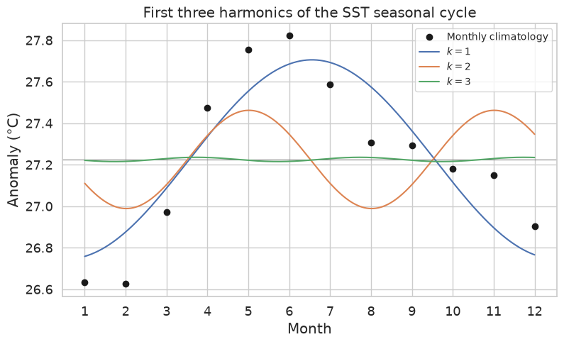

def reconstruct(y_mean, coeffs, t_eval, n, k_max):
    """Sum of the first k_max harmonics evaluated at times t_eval."""
    out = np.full_like(np.asarray(t_eval, dtype=float), y_mean)
    for k in range(1, k_max + 1):
        A, B, *_ = coeffs[k]
        out += A * np.cos(2 * np.pi * k * t_eval / n) \
             + B * np.sin(2 * np.pi * k * t_eval / n)
    return out


fig, ax = plt.subplots(figsize=(9, 4.5))
ax.plot(t, y, "ko", label="Monthly climatology")
for k_max, style in zip([1, 2, 3], ["-", "--", "-."]):
    ax.plot(
        t_fine,
        reconstruct(y_mean, coeffs, t_fine, n, k_max),
        style,
        label=f"Sum of {k_max} harmonic(s)",
    )
ax.set_title("Cumulative harmonic reconstruction (Wilks Fig. 10.15b analogue)")
ax.set_xlabel("Month, $t$")
ax.set_ylabel("SST (°C)")
ax.set_xticks(np.arange(1, 13))
ax.legend(loc="upper right", fontsize=10)
plt.show()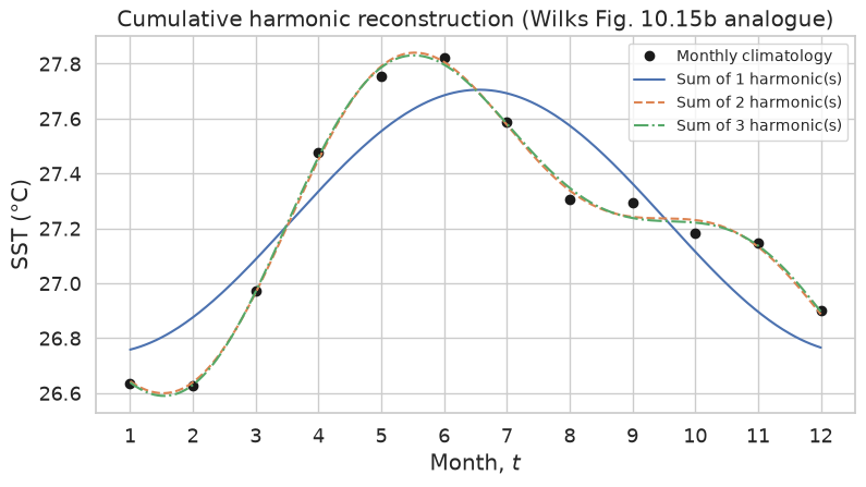

As we add more harmonics, the reconstruction converges to the data.

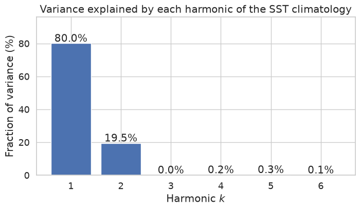
Variance explained by each harmonic¶

For an evenly-spaced series the variance contributed by harmonic $k$ is $C_k^2 / 2$ , and the total sample variance can be decomposed as

\operatorname{Var}(y) \;=\; \sum_{k=1}^{n/2} \frac{C_k^{\,2}}{2}.

(8)

This is Parseval’s identity for a finite cosine series, and it is the discrete analogue of the power spectrum introduced in the ---- notebook. Plotting $C_k^2/(2 \operatorname{Var}(y))$ tells us how much of the seasonal cycle’s variability is captured by each harmonic individually.

ks       = np.array(list(coeffs.keys()))
power_k  = np.array([C ** 2 / 2.0 for _, _, C, _ in coeffs.values()])
var_data = float(np.var(y, ddof=0))
frac     = power_k / var_data

print(f"Total sample variance  = {var_data:.4f}")
print(f"Sum of C_k^2 / 2       = {power_k.sum():.4f}  "
      f"(should equal the variance — Parseval)")

fig, ax = plt.subplots(figsize=(8, 4))
bars = ax.bar(ks, frac * 100, color=sns.color_palette("deep")[0])
ax.set_xlabel("Harmonic $k$")
ax.set_ylabel("Fraction of variance (%)")
ax.set_title("Variance explained by each harmonic of the SST climatology")
ax.set_xticks(ks)
for x, f in zip(ks, frac):
    ax.text(x, f * 100 + 1, f"{f * 100:.1f}%", ha="center")
ax.set_ylim(top=max(frac * 100) * 1.2)
plt.show()

Total sample variance  = 0.1439
Sum of C_k^2 / 2       = 0.1439  (should equal the variance — Parseval)

Exact reconstruction with all $n/2$ harmonics¶

With $n = 12$ samples the sum of $n/2 = 6$ harmonics has $2 \times 6 = 12$ free parameters — exactly enough to pass through every data point. This is an overfit in the previous regression analogy (one degree of freedom per data point), but here that is precisely the goal: we are representing the climatology, not forecasting future values.

full_recon = reconstruct(y_mean, coeffs, t, n, n // 2)

fig, ax = plt.subplots(figsize=(8, 4))
ax.plot(t, y, "ko", markersize=9, label="Data")
ax.plot(t, full_recon, "rx", markersize=12, mew=2,
        label=fr"Sum of all $n/2 = {n // 2}$ harmonics")
ax.set_title("All $n/2$ harmonics reproduce the data exactly")
ax.set_xlabel("Month, $t$")
ax.set_ylabel("SST (°C)")
ax.set_xticks(np.arange(1, 13))
ax.legend()
plt.show()

print(f"Max |reconstruction − data| = {np.max(np.abs(full_recon - y)):.2e} °C")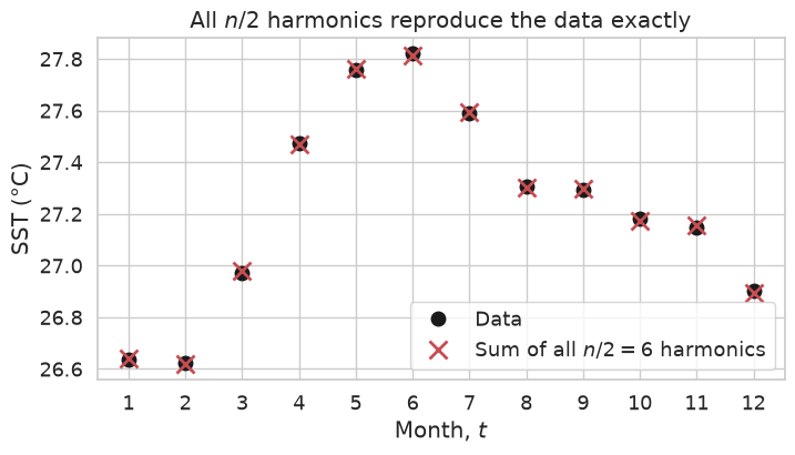

Max |reconstruction − data| = 6.59e-03 °C

Summary¶

Using single Sea Surface Temperature grid point, we were able to reconstruct the monthly seasonal cycle of the time series using Harmonic Analysis. Hee we showed that:

A single cosine wave with eyeballed amplitude and phase already captures the main features of the seasonal cycle.
Replacing the eyeballed values with least-squares estimates via the analysis equations tightens the fit, especially for the phase.
Higher harmonics extend the representation to any shape; the cumulative reconstruction with 1, 2, 3, … harmonics converges toward the data.
Summing all $n/2$ harmonics reproduces the climatology exactly.
The fraction of variance carried by each harmonic, $C_k^{\,2}/(2\sigma_y^2)$ , is a discrete line spectrum, the conceptual seed of the power spectrum studied in the --- notebook.

What’s next?¶

TBD

References¶

Wilks, D. S. (2019). Statistical Methods in the Atmospheric Sciences: An Introduction (4th ed). Elsevier.
Reynolds, R. W., Smith, T. M., Liu, C., Chelton, D. B., Casey, K. S., & Schlax, M. G. (2007). Daily high-resolution-blended analyses for sea surface temperature. Journal of Climate, 20(22), 5473–5496.