Skew T Diagrams

Overview

Skew-T plots are effectively thermodynamic diagrams used in meteorology. They display data collected from radiosonde balloons collecting atmospheric data including pressure level, temperature, relative humidity, and wind speed and direction.

In this notebook, we’ll learn about the structural and data components of Skew-T diagrams and how to plot them in Python using the MetPy package.

1. Elements of a Skew-T Diagram

2. Acquiring Sounding Data

3. Making a Skew-T plot in Python (with MetPy!)

Prerequisites

Concepts	Importance	Notes
Matplotlib	Necessary
Metpy	Useful

• Time to learn: 10 minutes

---

Elements of a Skew-T Plot

Let’s start out by talking about the structural elements of a Skew-T plot.

1. Temperature Lines are drawn at an angle up from the x-axis and are where the name “Skew-T” comes from.

2. Pressure Lines are horizontal from the y-axis, where pressure is plotted at a logarithmic scale.

3. Dry Adiabats: are lines of constant potential temperature as hypotethical air with no moisture content rises isentropically (with constant entropy).

4. Moist Adiabats: are lines of constant equivalent potential temperature - the change in temperature of fully saturated air as it rises, undergoing cooling due to adiabatic expansion.

5. Mixing Ratio Lines: represent lines of constant mixing ratio, the mass of water vapor relative to the mass of dry air.

On all those structural elements, Skew-T plots have two lines plotted on them, air temperature and dew point. In this notebook, we’ll be plotting the air temperature in red and the dew point in blue.

Additionally, Skew-T plots have wind barbs. These describe the wind speed and direction at different pressure levels and are plotted on the right side of the diagram.

Tip

For a more detailed description and a cool interactive diagram, visit NOAA’s Skew-T page.

import matplotlib.pyplot as plt
from mpl_toolkits.axes_grid1.inset_locator import inset_axes
import pandas as pd

from metpy.plots import SkewT, Hodograph
import metpy.calc as mpcalc
from metpy.units import units

Acquiring Sounding Data

If you want to get your own sounding data, run the following code in a new cell using the date and station of your choice:

from datetime import datetime
from siphon.simplewebservice.wyoming import WyomingUpperAir

date = datetime(2023, 7, 7, 0)
station = 'JAX'
df = WyomingUpperAir.request_data(date, station)

We’ve already done this for you and saved the data in a file, notebooks/data/jax_sounding.csv for you to use. We’ll use that file’s data for the rest of the notebook

df = pd.read_csv('data/jax_sounding.csv')
df

	pressure	height	temperature	dewpoint	direction	speed	u_wind	v_wind	station	station_number	time	latitude	longitude	elevation	pw
0	1012.0	9.0	24.8	23.6	0	0	0.000000	0.000000	JAX	72206	2023-07-07	30.5	-81.7	9.0	58.42
1	1003.0	88.0	26.3	22.6	210	14	7.000000	12.124356	JAX	72206	2023-07-07	30.5	-81.7	9.0	58.42
2	1000.0	115.0	26.8	22.2	210	14	7.000000	12.124356	JAX	72206	2023-07-07	30.5	-81.7	9.0	58.42
3	993.0	177.0	26.8	21.8	200	14	4.788282	13.155697	JAX	72206	2023-07-07	30.5	-81.7	9.0	58.42
4	986.0	240.0	26.6	20.8	190	14	2.431074	13.787309	JAX	72206	2023-07-07	30.5	-81.7	9.0	58.42
...	...	...	...	...	...	...	...	...	...	...	...	...	...	...	...
130	11.0	30681.0	-45.0	-79.0	70	29	-27.251086	-9.918584	JAX	72206	2023-07-07	30.5	-81.7	9.0	58.42
131	10.4	31057.0	-44.3	-78.3	79	33	-32.393697	-6.296697	JAX	72206	2023-07-07	30.5	-81.7	9.0	58.42
132	10.0	31320.0	-44.7	-78.7	85	36	-35.863009	-3.137607	JAX	72206	2023-07-07	30.5	-81.7	9.0	58.42
133	9.4	31735.0	-43.7	-77.7	85	37	-36.859204	-3.224762	JAX	72206	2023-07-07	30.5	-81.7	9.0	58.42
134	9.0	NaN	NaN	NaN	85	37	-36.859204	-3.224762	JAX	72206	2023-07-07	30.5	-81.7	9.0	58.42

135 rows × 15 columns

h = df['height'].values
p = df['pressure'].values
T = df['temperature'].values
Td = df['dewpoint'].values
u = df['u_wind'].values
v = df['v_wind'].values

Making a Skew-T plot in Python (with MetPy!)

So, all of that might seem a little abstract without a visual. We’re going to use MetPy’s SkewT module to make an actual Skew-T plot with the sounding data we downloaded earlier.

From the MetPy documentation:

“This class simplifies the process of creating Skew-T log-P plots in using matplotlib. It handles requesting the appropriate skewed projection, and provides simplified wrappers to make it easy to plot data, add wind barbs, and add other lines to the plots (e.g. dry adiabats)”

Just the basics

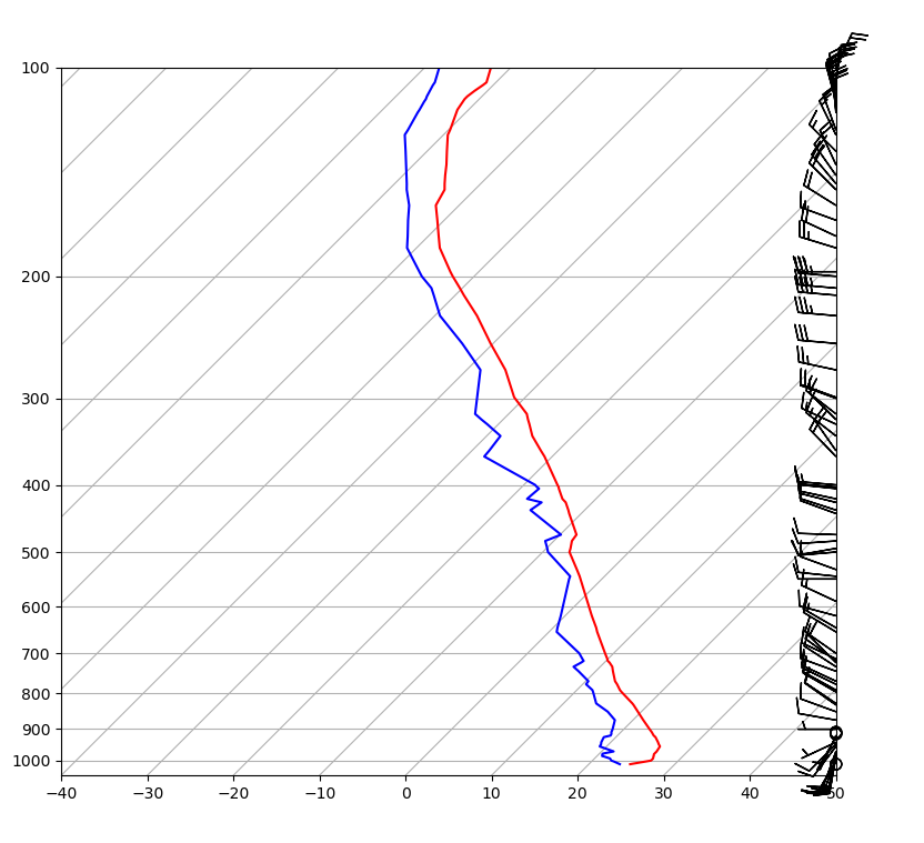
To start with, let’s create a very minimal Skew-T plot with just the pressure and temperature lines under the sounding data.

# make figure and `SkewT` object
fig = plt.figure(figsize=(9, 9))
skewt = SkewT(fig=fig, rotation=45)

# plot sounding data
skewt.plot(p, T, 'r')  # air temperature
skewt.plot(p, Td, 'b')  # dew point
skewt.plot_barbs(p[p >= 100], u[p >= 100], v[p >= 100])  # wind barbs

<matplotlib.quiver.Barbs at 0x7fd460c7db10>

Let’s talk break that down a bit.

# make figure and `SkewT` object
fig = plt.figure(figsize=(9, 9))
skewt = SkewT(fig=fig, rotation=45)

First, we made a new figure and used it to make a new skew-T plot. If you don’t provide a figure to SkewT, one will be created for you, but it’s useful to make the default figure size a bit larger for this tutorial.

Additionally, we’ve also set the rotation kwarg to be 45 degrees. This is the angle that the temperature lines will be drawn at. MetPy’s default is 30 degrees, but we’re going to use a more traditional 45 degrees for this tutorial.

# plot sounding data
skewt.plot(p, T, 'r') # air temperature
skewt.plot(p, Td, 'b') # dew point

For air temperature and dew point, we can use the standard plot method. The SkewT object provides a wrapper around matplotlib’s plot method, and can be used in the same way. Note that even though pressure is on the y-axis, we still provide it as the first argument to plot because it is the independent variable.

skewt.plot_barbs(p[p >= 100], u[p >= 100], v[p >= 100]) # wind barbs

Finally, we use SkewT’s plot_barbs method to add the wind barbs to the right side of the plot. This is a wrapper around matplotlib’s barbs method that applies the appropriate transformation and positions the barbs as expected for a Skew-T plot. Note that we only plot the wind barbs for pressure levels greater than 100 hPa. This is just to keep the wind barbs from extending off the plot.

In addition to the elements we have added specifically, you can see that the SkewT object also added some of the structural elements we discussed previously. By default, SkewT adds the horizontal pressure and skewed temperature lines.

Adding more structural elements

Next, let’s add the rest of the structural elements to the plot.

# make figure and `SkewT` object
fig = plt.figure(figsize=(9, 9))
skewt = SkewT(fig=fig, rotation=45)

# plot sounding data
skewt.plot(p, T, 'r') # air temperature
skewt.plot(p, Td, 'b') # dew point
skewt.plot_barbs(p[p >= 100], u[p >= 100], v[p >= 100])  # wind barbs

# add dry adiabats, moist adiabats, and mixing ratio lines
skewt.plot_dry_adiabats()
skewt.plot_moist_adiabats()
skewt.plot_mixing_lines()

<matplotlib.collections.LineCollection at 0x7fd4615fff10>

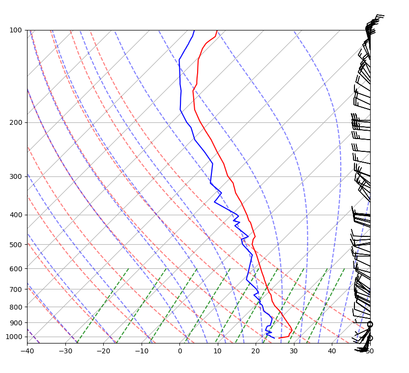
Similarly to the plot_barbs command, the SkewT object provides convenient methods for adding the remaining structural elements to the plot.

The default appearance of these elements is:

• Dry Adiabats: dashed red/pinkish lines with an alpha value of 0.5

• Moist Adiabats: dashed blue lines with an alpha value of 0.5

• Mixing Ratio Lines: dashed green lines with an alpha value of 0.8

These defaults can be overwritten by providing additional keyword arguments to the methods.

Polishing the plot

Now that we have all the structural elements on the plot, let’s make it look a little nicer. The previous plot has all the necessary information, but it’s a little cluttered and hard to read.

# make figure and `SkewT` object
fig = plt.figure(figsize=(8,12))
skewt = SkewT(fig=fig)
skewt.ax.set_ylim(1000, 10)

# plot sounding data
skewt.plot(p, T, 'r') # air temperature
skewt.plot(p, Td, 'b') # dew point
skewt.plot_barbs(p[::5], u[::5], v[::5]) # add a wind barb every fifth level

# add dry adiabats, moist adiabats, and mixing ratio lines
skewt.plot_dry_adiabats(linewidth=0.5)
skewt.plot_moist_adiabats(linewidth=0.5)
skewt.plot_mixing_lines(linewidth=0.5)

# add axis and figure titles
plt.title(df['station'][0] + ' ' + str(df['time'][0]))
plt.xlabel('temperature (degC)')
plt.ylabel('pressure (hPa)')

Text(0, 0.5, 'pressure (hPa)')

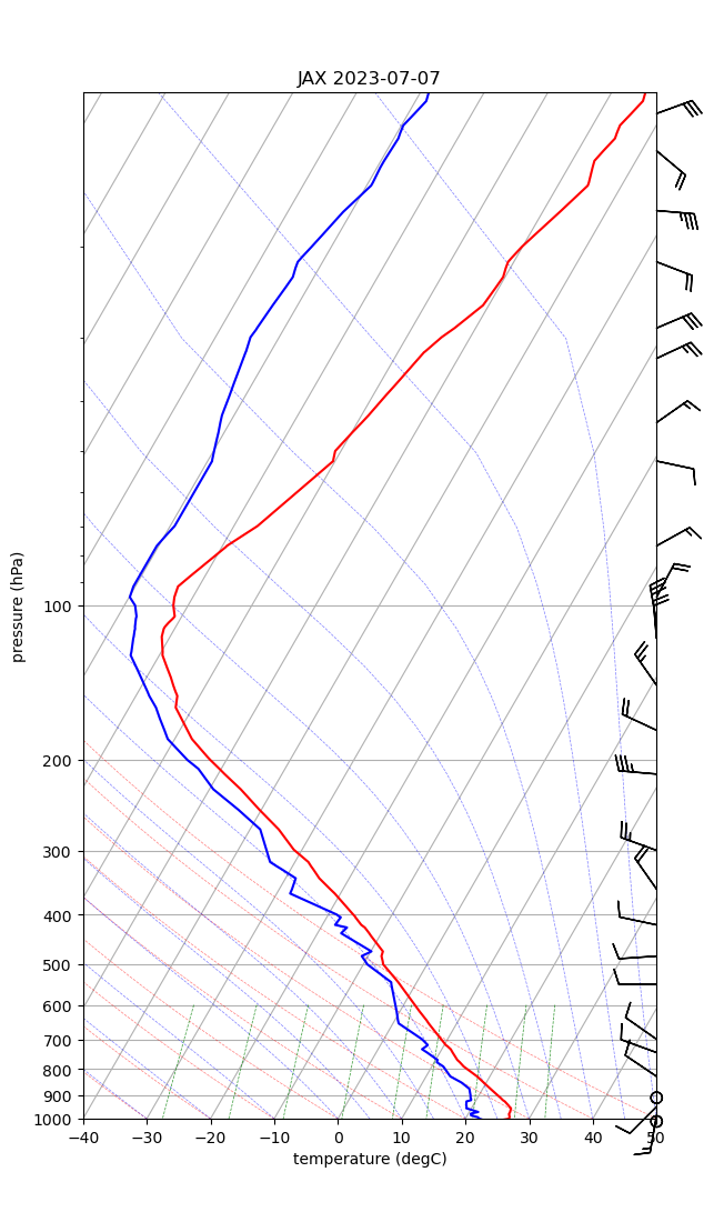
Here, we’ve made the following changes:

• changed the figsize to figsize=(8,12)

• removed the rotation kwarg from the SkewT object to allow the upper air temp and dew point lines to be seen without being cut off or expanding the x-axis limits

• skewt.ax.set_ylim(1000, 10): sets the y-axis limits to 1000 hPa at the bottom and 10 hPa at the top to include the entire sounding

• skewt.plot_barbs(p[::5], u[::5], v[::5]): plots every fifth wind barb to reduce clutter, also removes limiting the wind barbs to pressure levels greater than 100 hPa

• reduced the linewidth of the dry adiabats, moist adiabats, and mixing ratio lines to 0.5

• added axes labels

• added a title including the station name and date of the sounding pulled from the data

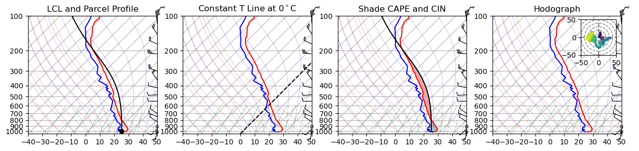
Additional Skew-T Options

There are a few additional options that can be used to customize the appearance of the Skew-T plot that we haven’t covered here. For more information, check out the MetPy documentation.

Here’s a few quick examples of some of those additional options:

fig = plt.figure(figsize=(15, 4))

# set up some subplots
skewt_plots = []
for i in range(0,4):
    skewt_plots.append(SkewT(fig=fig, subplot=(1,4,i+1), rotation=45))
    skewt_plots[i].plot(p, T, 'r') # air temperature
    skewt_plots[i].plot(p, Td, 'b') # dew point
    skewt_plots[i].plot_barbs(p[::5], u[::5], v[::5], length=5, linewidth=0.5)
    skewt_plots[i].plot_dry_adiabats(linewidth=0.5)
    skewt_plots[i].plot_moist_adiabats(linewidth=0.5)
    skewt_plots[i].plot_mixing_lines(linewidth=0.5)
    skewt_plots[i].ax.set_xlabel('')
    skewt_plots[i].ax.set_ylabel('')

# calculate LCL and parcel profile
lcl_p, lcl_t = mpcalc.lcl(p[0]*units.hPa, T[0]*units.degC, Td[0]*units.degC)
lcl_prof = mpcalc.parcel_profile(p*units.hPa, T[0]*units.degC, Td[0]*units.degC).to('degC')


# LCL and parcel profile skew-T
# At what point an air parcel lifted as a dry parcel becomes saturated
skewt_plots[0].ax.set_title('LCL and Parcel Profile')
skewt_plots[0].plot(p, lcl_prof, 'k')
skewt_plots[0].plot(lcl_p, lcl_t, 'ko') # Lifted Condensation Level


# add constant temperature line at t=0
skewt_plots[1].ax.set_title('Constant T Line at 0$^\circ$C')
skewt_plots[1].ax.axvline(0, color='k', ls='--')


# shade CAPE and CIN
# Area above and below the Level of Free Convection  (LFC) - where the temeprature line crosses the moist adiabat
# Updraft energy for thunderstorms (CAPE) and energy needed for the storm to start (CIN)
skewt_plots[2].ax.set_title('Shade CAPE and CIN')
skewt_plots[2].plot(p, lcl_prof, 'k')
skewt_plots[2].shade_cin(p*units.hPa, T*units.degC, lcl_prof, Td*units.degC)  # Convective INhibition
skewt_plots[2].shade_cape(p*units.hPa, T*units.degC, lcl_prof) # Convective Available Potential Energy


# Hodograph
#  A line that connects the tips of wind vectors between two atmospheric heights
# # Used for understanding wind sheer
skewt_plots[3].ax.set_title('Hodograph')
ax_hod = inset_axes(skewt_plots[3].ax, '30%', '30%')
hod = Hodograph(ax_hod, component_range=50)
hod.add_grid(increment=10)
hod.plot_colormapped(u, v, h)

<matplotlib.collections.LineCollection at 0x7fd4588becd0>

Summary

Skew-T plots are a useful tool for visualizing and understanding sounding data. Creating Skew-T plots in python might seem challenging given their unique structural characteristics, but MetPy’s SkewT module greatly simplifies the process.

What’s next?

Next up let’s discuss spaghetti plots.

Resources and references

• Wyoming Upper Air

• Siphon

• MetPy’s SkewT documentation

• NOAA’s JetStream’s Skew-T Plot page