Contributors: Mike Durand
School of Earth Sciences and Byrd Polar & Climate Research Center durand.8@osu.edu
Learning Objectives
At the end of this tutorial you should be able to...
Explain why microstructure is important for remote sensing
Define measures of microstructure, especially specific surface area
Access and visualize tree different microstructure measurements from SnowEx Grand Mesa 2020
Caveats
The integrating sphere and the SMP data are published at NSIDC; you can read the pages there for documentation etc. However the microCT data are not yet published; please contact Lauren Farnsworth (lauren
Fun Facts About Snow Microstructure
Snow microstructure plays a super important role in snow physics and snow remote sensing, so a lot of effort went towards measuring it in SnowEx 2020!
There are several different quantities that are used to measure snow microstructure, including “grain size”. Grain size measurements are challenging to make in a repeatable way, and are also challenging to relate to the physical quantities that control remote sensing measurements. In the last ~15 years or so, a lot of effort has gone into more objective ways to measure microstructure.
Snow microstructure governs response of remote sensing to snow cover for visible, near-infrared and high-frequency microwave wavelengths. See Figure 1, below, and read Dozier et al., 2009, for more information.
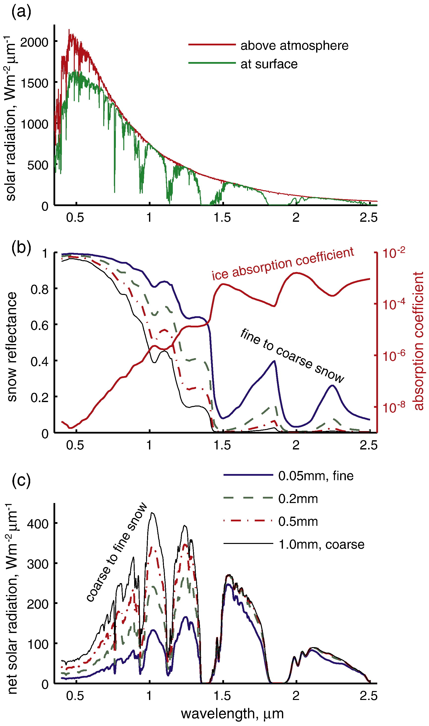
Snow microstructure governs visible and near-infrared reflectance. This is figure 2 from Dozier et al., 2009
Radar measurements such as those made by the Ku-band SWEARR instrument are also very sensitive to snow microstructure.
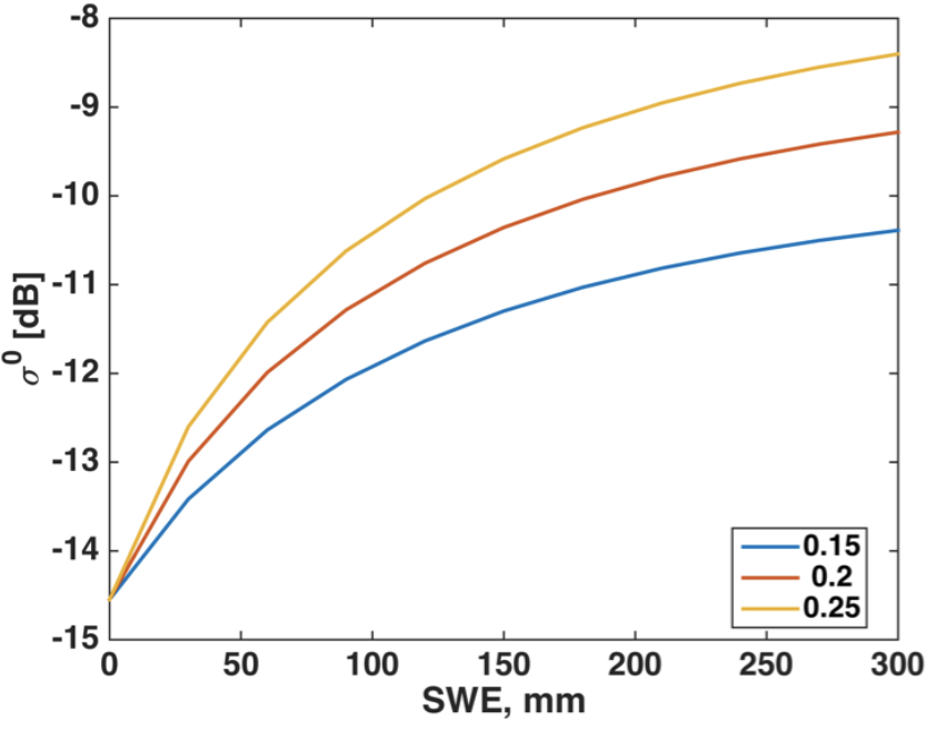
Modeled response of radar backscatter to SWE and single-scatter albedo (which in turn is a function of snow microstructure), based on a simple model suggested by Ulaby, 2014.
Snow microstructure is super important to efforts to launch a Ku-band SAR to measure global snow water equivalent (SWE). An important area of research right now is exploring how to use estimates of microstructure (e.g. from snowpack evolution models) to improve SWE retrievals.
Snow microstructure evolves through the season, and varies a lot with depth. Snow microstructure evolution is controlled by other snow properties, such as snow temperature, snow height and snow liquid water content. A really great resource on snow microstructure is Kelly Elder’s recent talks:
SnowEx Microstructure Measurement Background
Basic Microstructure Definitions
Microstructure definitions take a bit of getting used to. It’s very easy to get confused. Specific surface area (SSA) is one of the most important quantity used to measure snow microstructure, so that’s the focus here. Note that SSA is not the be-all and end-all, so there’s a short table describing how to relate SSA to other quantities just below. A couple of good reads on all of this is Mätzler, 2002 and Matzl & Schneebeli, 2010.
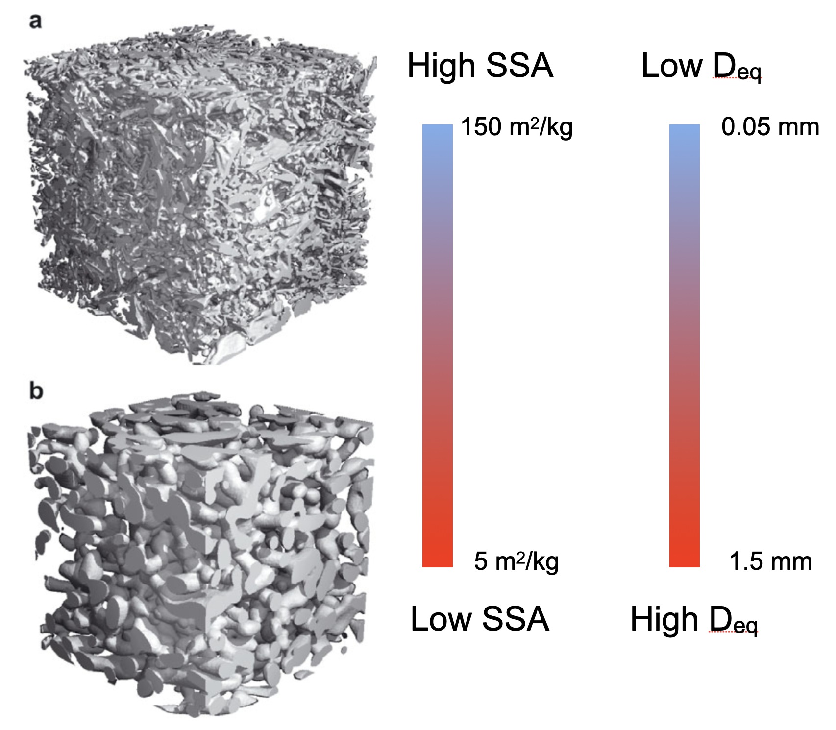
Coarse and fine snow microstructure revealed by microCT. The microCT snow renderings on the left are Figure 2 from Löwe et al., 2011. The colorbars indicate that fine-grained snow (a) has high SSA and low Deq, whereas coarse-grained snow (b) has low SSA and high Deq
Use Figure 3 above to ground these definitions: SSA is the surface area of the ice-air interface, normalized in some way. Confusingly, SSA is defined in a couple of different ways in the literature: sometimes, surface area within a particular volume of interest (VOI) is normalized by the mass of the ice in the VOI. As defined in this way, SSA has units of length squared per mass, usually expressed as m2/kg. Instead of normalizing by mass, SSA is sometimes defined by normalizing by the volume of the VOI (this is SSAv in Matzl & Schneebeli, 2010), and sometimes by normalizing by the volume of the ice in the VOI (this is SSAi in Matzl & Schneebeli, 2010, and q in Mätzler, 2002). Here let’s just go with the first definition I mentioned:
SSA tends to take values between 5 and 150 m2/kg: fresh, fine-grained snow has high SSA, and coarse snow has low SSA. Because it takes a little while for SSA values to become intuitive, a useful derived metric is the equivalent grain diameter (Deq; note that this is identical to Dq in Mätzler, 2002), which by definition is the diameter that a sphere would have if it had a particular value of SSA. This is a one-to-one relationship, so there are no assumptions involved.
Relationships of specific surface area to other metrics are given in this list if you’re curious but otherwise just skip past this bit
Sometimes people refer to the “optical grain diameter”, which is the same as Deq. The “optical” refers to Grenfell & Warren, 1999, who showed that any snow with a particular SSA had similar (not identical) radiative transfer properties regardless of particle shape in the visible and near-infrared parts of the spectrum. But note the same is not true in the microwave spectrum.
Autocorrelation length is usually one of two metrics that summarize the two-point microstructure autocorelation function of the three-dimensional ice-air matrix. Think of the probability that you change media (from ice to air or vice versa) as you move a certain distance within the snow microstructure. The length that defines the likelihood that you’ll change media is (an approximation of the correlation length). SSA is by definition (with almost no assumptions) equal to the slope of the autocorrelation function at the origin. But microwave scattering is controlled by correlations at longer lags. For more check out Mätzler, 2002. The lack of closing the loop between SSA and correlation length is a significant issue when we have measurements of SSA and microwaves as we do in SnowEx.
Geometric grain size is what we usually measure when we measure with a hand lens. You can try to relate it to SSA or corelation length, but it is not always possible, and will change with different observers.
Time to stop this list but there are many other metrics as well.
Microstructure Instruments
Now that we know what we’re trying to measure (SSA, or correlation length) how do we actually measure? let’s talk just about three techniques used in SnowEx 2020 Grand Mesa.
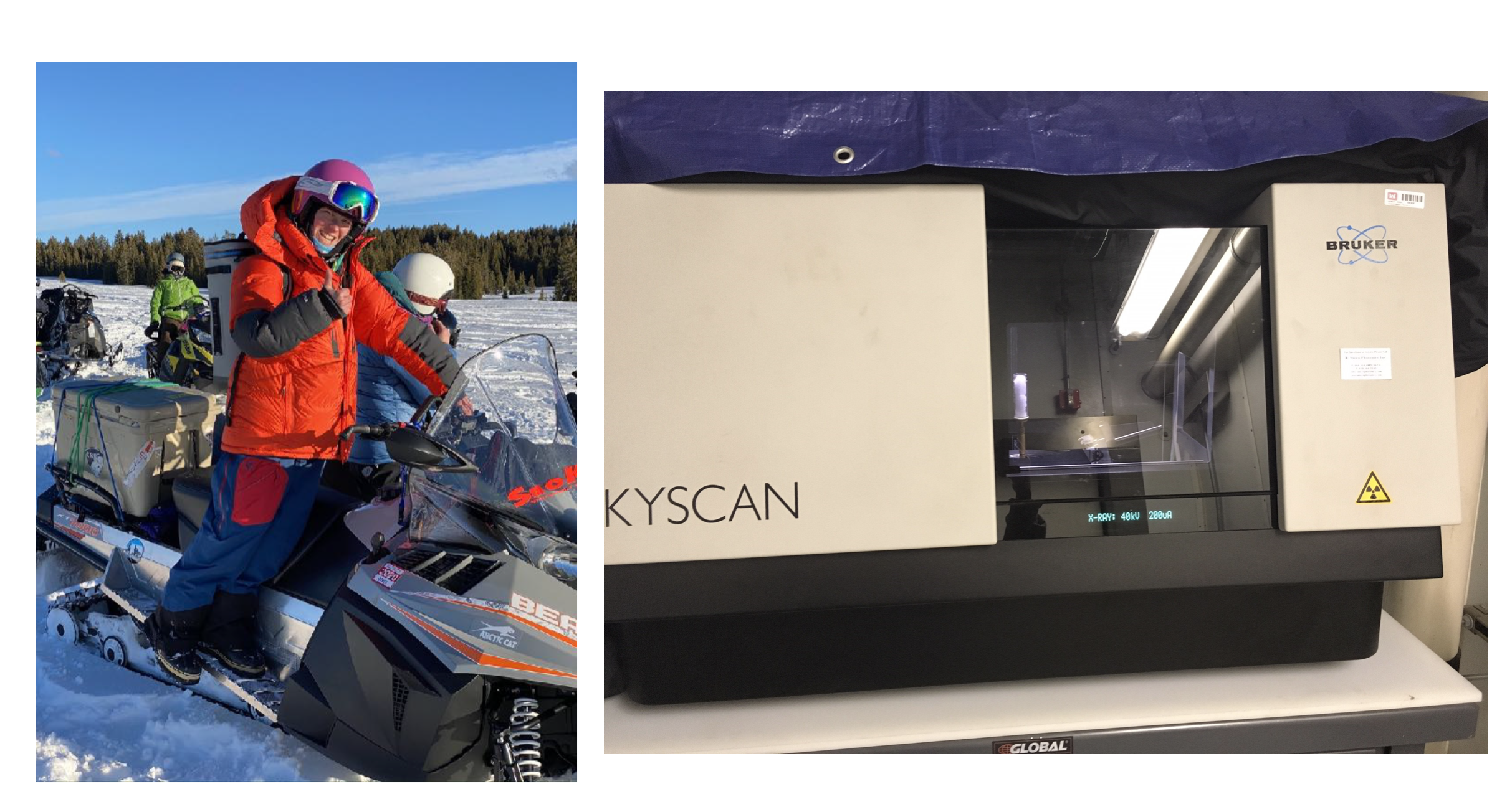
Left: Lauren Farnsworth transports microCT samples from field sites back to Grand Mesa Lodge in a cold storage container. Right: the microCT machine in the lab at CRREL.
Micro-computed tomography (microCT) is the only laboratory-based method used here, and it is the gold standard, although it does still come with caveats. The idea of microCT is to remove a sample of snow from a snow pit face, and either cast it with a compound such as diethyl pthalate that is still a liquid at 0° C, or preserve the same at a very cold temperature. Then the sample is sent back to the laboratory, and bombared with x-rays, similar to how you get x-rays to see if a bone is broken at the doctor. For much more on microCT, check out HEGGLI et al., 2011. microCT can be used to extract a ton of information about snow microstructure, including SSA, correlation length and many others.
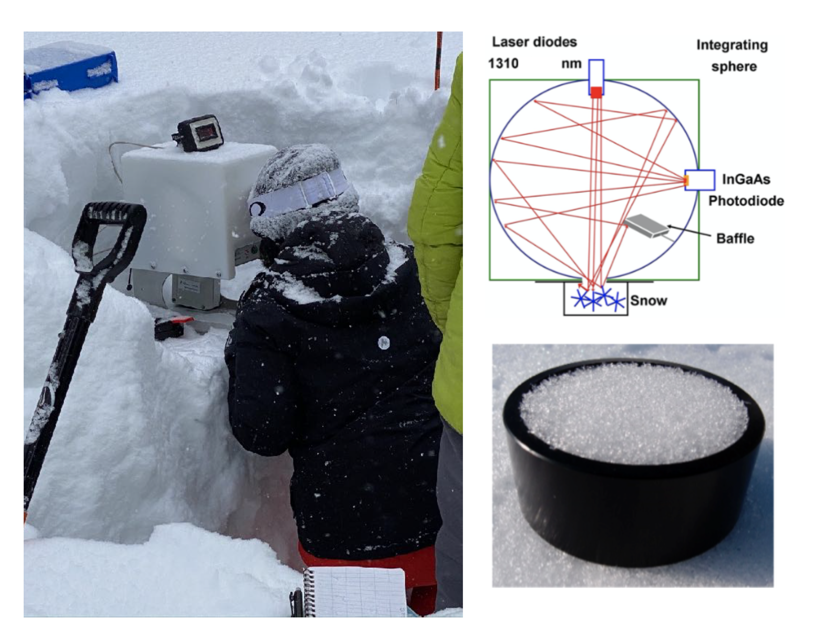
Left: Kehan Yang operates an IceCube unit at the Grand Mesa Lodge intercomparison snowpit. Top right: schematic showing the integrating sphere measurement principle, from Gallet et al., 2009. Bottom right: snow in the IceCube sampling container, from Leppänen & Kontu, 2018.
Integrating spheres are field-based and you make the measurements on samples extracted from the snowpit face. The principle of the measurement is based on firing a laser at the snow sample, within a special reflective hollow sphere, where one side is filled by the snow sample, and measuring how much of the laser is reflected at a sensor at a known geometry. For more information, check out Gallet et al., 2009. Most integrating sphere measurements are either made by a commercial firm (A2 Photonics) known as the IceCube or a version constructed at the University of Sherbrooke known as the IRIS Montpetit et al., 2012. These approaches are set up to measure SSA only. There were three of these at Grand Mesa - one of the Sherbrooke IRIS units, and two IceCubes, one from Finnish Meteorological Institute, and one from Ohio State University.
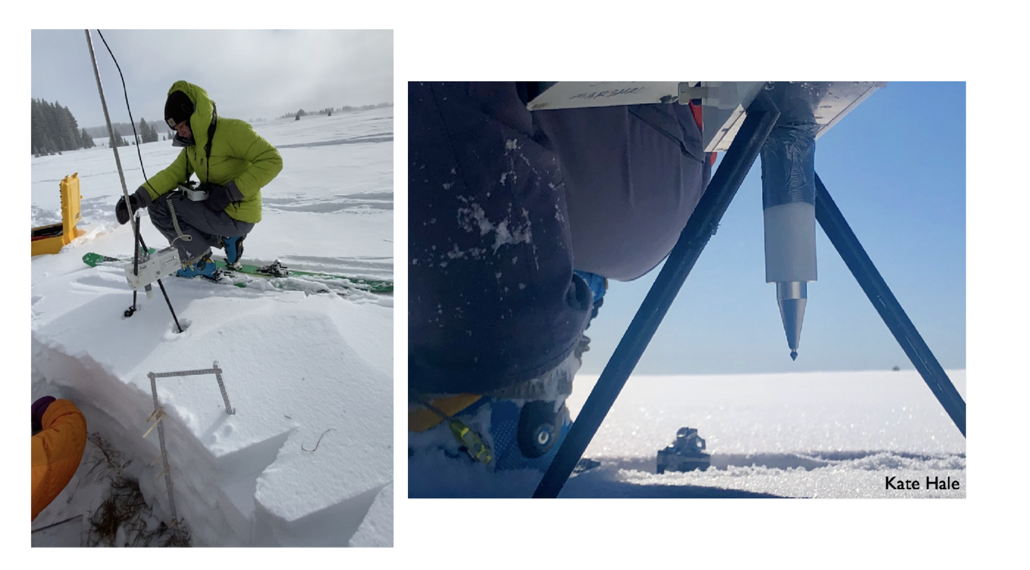
Left: Megan Mason operates the SMP. Right: Closeup of the SMP sensor tip.
Snow micropenetrometers are also a field-based approach, but they do not require a snowpit, enabling far more observations to be made. Instead, an automated motor pushes a probe vertically downwards into the snowpack. The probe measures the force required to break snow microstructure, yielding a wealth of information. Snow density, specific surface area and correlation length can be retrieved; for background see Löwe & Herwijnen, 2012 and Proksch et al., 2015. The micropen effort at Grand Mesa was led by Boise State University. A key thing to be aware of is that differences in the various SMP instruments mean that the empirical relationship of Proksch et al., 2015 will give quite poor results for the particular instrument used in SnowEx, as fully explained in Calonne et al., 2020.
These methods are not the only ways to measure microstructure! There are several others not mentioned here, but not used at Grand Mesa 2020. Ask if interested.
SnowEx Microstructure Measurement Data Overview
Of the three methods described above, microCT is by far the most expensive and most time consuming. Samples have to be transported back to the laboratory and the processing time requires a microCT machine. Thus the fewest CT sapmles are taken.
The integrating spheres require a snowpit to be dug, so we have an intermediate number of them: ~100.
The micropen measurements are by far the fastest to make, so a cross pattern of SMP measurements was made on orthogonal directions intersecting at the snowpit. There are thousands of SMP profiles from Grand Mesa 2020.
Working with the data
We’re going to do two things! First, we’ll intercompare the three different integrating sphere instruments at four different pits where we had multiple instruments operating. We’d expect these data to be fairly self-consistent. Second, we’ll compare all three methods (integrating sphere, SMP and microCT) at a single pit where we had all of these measurements present. Here especially with the SMP we would expect to need to intercalibrate the data to match local conditions; so far SSA has only been fit to SMP force measurements in one study, and we should assume we’ll need a local calibration to get a tight fit.
0. Load needed modules
from snowexsql.lambda_client import SnowExLambdaClient

# Modules needed to work with data
import matplotlib.pyplot as plt
import pandas as pd
import numpy as np
import contextily as cx

from snowmicropyn import Profile
from snowmicropyn import proksch2015

import os
import warnings
warnings.filterwarnings('ignore')
# Initialize client
client = SnowExLambdaClient()
# Get all measurement classes dynamically
classes = client.get_measurement_classes()
LayerMeasurements = classes['LayerMeasurements']
print("🔍 Testing Lambda connection...")
connection_test = client.test_connection()
print(f"✅ Connected: {connection_test.get('connected', False)}")
if connection_test.get('connected'):
print(f"📊 Database: {connection_test.get('version', 'Unknown version')}")
else:
print("❌ Connection failed")🔍 Testing Lambda connection...
✅ Connected: True
📊 Database: PostgreSQL 16.10 on x86_64-conda-linux-gnu, compiled by x86_64-conda-linux-gnu-cc (conda-forge gcc 14.3.0-4) 14.3.0, 64-bit
1. Intercompare Integrating Sphere Datasets
There were three integrating spheres. The IRIS unit from University of Sherbrooke was operated by Celine Vargel. The IceCube unit from the Finnish Meteorological Institute was operated by Juha Lemmetyinen. And the IceCube unit from Ohio State was operated by Kehan Yang and Kate Hale. Carefully read the documentation page at NSIDC if you are interested in the data. If you are using the data for a project, please contact the authors and mention what you’re doing - they’ll appreciate it! Contact for SSA is Mike Durand (durand.8@osu.edu).
SSA = LayerMeasurements.from_filter(
    type='specific_surface_area',
    limit=3000,
    verbose=True
)

SSA.head() #check out the results of the querySince we want to intercompare integrating spheres, we need to isolate only the sites that actually had multiple integrating spheres measuring the same snow.
# Grab all the sites with equivalent diameter data (set reduces a list to only its unique entries)
sites = SSA['site_name'].unique()
# Store all site names that have multiple SSA instruments
multi_instr_sites = []
instruments = []
for site in sites:
# Grab all the layers associated to this site
site_data = SSA.loc[SSA['site_name'] == site]
# Do a set on all the instruments used here
instruments_used = site_data['instrument_name'].unique()
if len(instruments_used) > 1:
multi_instr_sites.append(site)
# Get a unqique list of SSA instruments that were colocated
instruments = SSA['instrument_name'].unique()
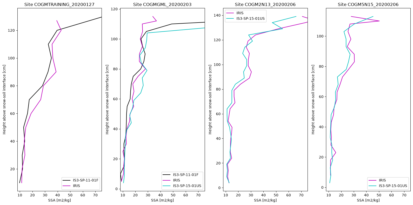
instruments #check out the list of instruments. note that the IceCube values are displayed as serial numbersarray(['IS3-SP-11-01F', 'IRIS', 'IS3-SP-15-01US'], dtype=object)Finally, plot all Integrating Sphere SSA profiles at all Multi-Integrating Sphere Sites
# Setup the subplot for each site for each instrument
fig, axes = plt.subplots(1, len(multi_instr_sites), figsize=(4*len(multi_instr_sites), 8))

# Establish plot colors unique to the instrument
c = ['k', 'm', 'c']
colors = {inst:c[i] for i,inst in enumerate(instruments)}

# Loop over all the multi-instrument sites
for i, site in enumerate(multi_instr_sites):

    # Grab the plot for this site
    ax = axes[i]

    # Loop over all the instruments at this site
    for instr in instruments:

        # Grab our profile by site and instrument
        ind = SSA['site_name'] == site
        ind2 = SSA['instrument_name'] == instr
        profile = SSA.loc[ind & ind2].copy()

        # Don't plot it unless there is data
        if len(profile.index) > 0:

            # Sort by depth so samples that are take out of order won't mess up the plot
            profile = profile.sort_values(by='depth')

            # Layer profiles are always stored as strings.
            profile['value'] = profile['value'].astype(float)

            # Plot our profile
            ax.plot(profile['value'], profile['depth'], colors[instr], label=instr)

    # Labeling and plot style choices
    ax.legend()
    ax.set_xlabel('SSA [m2/kg]')
    ax.set_ylabel('Height above snow-soil interface [cm]')
    ax.set_title('Site {}'.format(site.upper()))

    # Set the x limits to show more detail
    ax.set_xlim((8, 75))

plt.tight_layout()
plt.show()
2. Pull the snowmicropenetrometer data and compute SSA
The next step is to grab some SMP data to compare to. We’re going to get the SMP at site 2N13, where we have a copule of SSA profiles from integrating spheres (as well as microCT data, to be looked at in the next step!).
The SMP measurements for SnowEx 2020 GrandMesa were all made by Megan Mason. If you’re interested in working with the SMP data, please carefully read the NSIDC documentation page. If you’re planning to work with the data, please reach out to the author; the contact is (Megan Mason megan
As mentioned above, Calonne et al., 2020 tested applying the relationship of Proksch et al., 2015 and got quite poor results, explained them by the difference in hardware between generations of SMP instruments. We were unaware of that when designing the tutorial, and so set up use of the so-called official SMP processing repository, linked below, which has not yet been updated with the latest relationship. This would make a great project, as mentioned later!
First up, we’ll visualize the location of the SMP profiles, along with the snowpit location. All the data we will be working with is associated with the site label ‘2N13’. We’ll begin by querying all site names in the database and look for that string. We’ll use the get_sites method in the SnowEx API that provides basic information on the name and location of all layer measurement sites.
# Get all sites containing '2N13'
sites_with_2N13 = [site for site in LayerMeasurements.all_sites if '2N13' in site]
print(f"Found {len(sites_with_2N13)} sites containing '2N13':")
siteLocations = LayerMeasurements.get_sites(site_names=sites_with_2N13)
siteLocations
Found 16 sites containing '2N13':
The site labeled COGM2N13_20200206 refers to the snowpit location, while the remaining 15 sites are SMP observations.
Next we will plot the locations of these observations to assess their spatial proximity:
# Separate the pit location from SMP locations
pit_location = siteLocations[siteLocations['name'] == 'COGM2N13_20200206']
smp_locations = siteLocations[siteLocations['name'] != 'COGM2N13_20200206']

# Convert to Web Mercator for basemap
smp_locations_wm = smp_locations.to_crs(epsg=3857)
pit_location_wm = pit_location.to_crs(epsg=3857)

# Create the plot
fig, ax = plt.subplots(figsize=(10, 10))
smp_locations_wm.plot(ax=ax, marker='o', color='orange', markersize=100, edgecolor='black', label='SMP Locations')
pit_location_wm.plot(ax=ax, marker='s', color='black', markersize=150, edgecolor='black', label='Pit Location')

# Add labels for SMP locations
for idx, row in smp_locations_wm.iterrows():
    ax.annotate(row['name'],
                xy=(row.geometry.x, row.geometry.y),
                xytext=(5, 5),
                textcoords='offset points',
                fontsize=6,
                bbox=dict(boxstyle='round,pad=0.3', facecolor='white', alpha=0.7, edgecolor='none'))

# Add label for pit location
for idx, row in pit_location_wm.iterrows():
    ax.annotate(row['name'],
                xy=(row.geometry.x, row.geometry.y),
                xytext=(5, 5),
                textcoords='offset points',
                fontsize=6,
                bbox=dict(boxstyle='round,pad=0.3', facecolor='white', alpha=0.7, edgecolor='none'))

# Zoom out by adding buffer to axis limits
xlim = ax.get_xlim()
ylim = ax.get_ylim()
x_buffer = (xlim[1] - xlim[0]) * 0.5
y_buffer = (ylim[1] - ylim[0]) * 0.5
ax.set_xlim(xlim[0] - x_buffer, xlim[1] + x_buffer)
ax.set_ylim(ylim[0] - y_buffer, ylim[1] + y_buffer)

# Add basemap - using Esri World Imagery for satellite view with terrain
cx.add_basemap(ax, source=cx.providers.Esri.WorldImagery, alpha=0.5)

# Avoid using Scientific notation for coords
ax.ticklabel_format(style='plain', useOffset=False)

ax.set_xlabel('Easting [m]', fontsize=12)
ax.set_ylabel('Northing [m]', fontsize=12)
ax.set_title('Site Locations', fontsize=14)
ax.legend()
plt.tight_layout()
plt.show()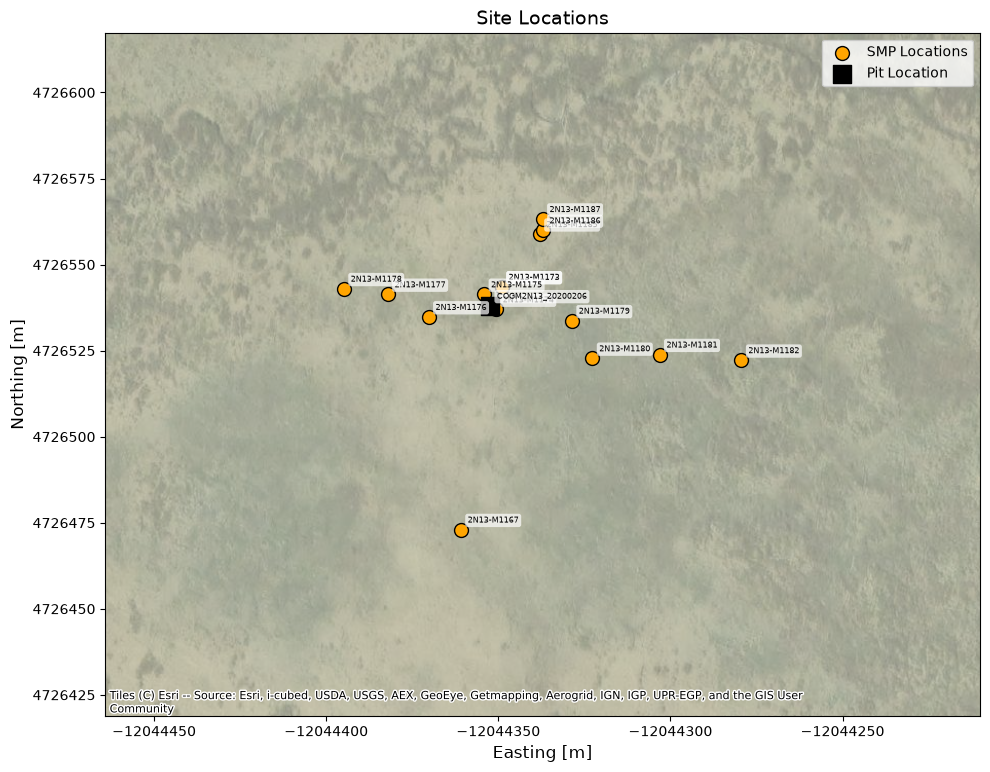
Next up, let’s find the closest SMP profile to the snowpit, and then find the profile ID of that profile, which is in the comments in the database.
# Find the closest SMP location to the pit
from shapely.geometry import Point

# Get pit coordinates
pit_coords = pit_location.geometry.values[0]

# Calculate distance from each SMP location to the pit
smp_locations['distance_to_pit'] = smp_locations.geometry.apply(lambda x: x.distance(pit_coords))

# Find the closest SMP location
closest_smp = smp_locations.loc[smp_locations['distance_to_pit'].idxmin()]

print(f"Closest SMP location to pit: {closest_smp['name']}")
print(f"Distance: {closest_smp['distance_to_pit']:.2f} meters")
Closest SMP location to pit: 2N13-M1174
Distance: 0.00 meters
So the id of the closest SMP profile is 2N13-M1174.
Now we’ll work on acquiring the associated data. Note that the SMP datasets are quite large and store a suite of observations. The SnowEx database currently stores a subset of the data, the force and depth profiles, but the remaining observations are not yet in the database. So for this exercise we will need to download the raw output from the sensor and do some additional processing.
To do this we go to the SMP page on NSIDC, choose “Download” and searched for the 2N13-M1174 ID. We’ve downloaded two raw point files, located in the data\microstructure\SMP directory in this repository, just for the sake of this tutorial.
Now we have to compute SSA from the SMP data. For this, we’ll use the “snowmicropyn” modules created by the Swiss SLF. You can read more about them at this site. The software is a little out of date on Python versions; just ignore any warnings that pop up below! Also, the use of the Proksch et al., 2015 relationship is also out-of-date, as mentioned above.
p = Profile.load('data/microstructure/SMP/SNEX20_SMP_S19M1174_2N13_20200206.PNT',)
plt.plot(p.samples.distance, p.samples.force)
# Prettify our plot a bit
plt.title(p.name)
plt.ylabel('Force [N]')
plt.xlabel('Depth [mm]')
plt.show()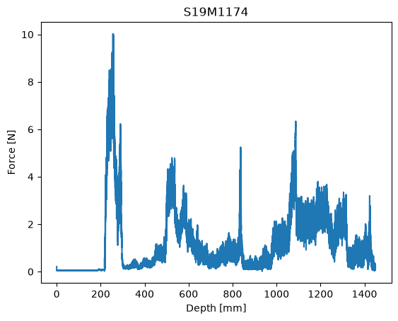
The above shows the entire SMP profile; this includes the part of the force profile that is above the snow surface, and thus needs to be removed, in order to apply calculations only to the snow (not the air!).
#extract the part of the profile that is in the snow (i.e. remove air)
depth_surf=p.detect_surface()
depth_ground=p.detect_ground()
samples_snow=p.samples_within_distance(begin=depth_surf, end=depth_ground, relativize=False)
samples_snow.distance-=depth_surf
plt.plot(samples_snow.distance, samples_snow.force)
plt.title(p.name)
plt.ylabel('Force [N]')
plt.xlabel('Depth [mm]')
plt.show()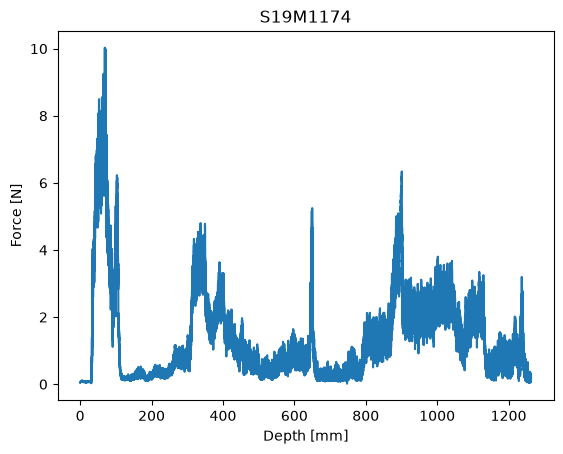
The above part of the profile is just the part that is in the snow. PLEASE NOTE that the automated functions are not infallible, and need to be used with care. For now, these need to be compared back to the notes and interpreted manually.
The next step is the actual calculation of SSA from the force data. It then displays the data and lets you see that there is now a column called SSA! Note that this function is “proksch2015”. You can read about how it works in Martin Proksch’s paper Proksch et al., 2015.
# call using the snowmicropyn library proksch2015
p2015 = proksch2015.calc(p.samples)
p2015.head() #check out the first few values of SSA3. Read microCT data, and compare integrating sphere, SMP and CT data
The microCT samples were extracted in the field and processed at CRREL by Lauren Farnsworth, and is not yet published at NSIDC. Please contact her with questions (lauren
This module reads in microCT datafiles which are stored as text. Some additional data are available, showing the computer generated slices through the ice-air interface: contact Mike (durand.8@osu.edu) if you want to look at a subset of these data that Lauren has shared.
Equivalent grain size is a useful quantity to compare: because it’s proportional to 1/SSA, and because after a point as you increase SSA more and more, all fine-grained snow acts more-or-less the same (converging to e.g. the “fine-grained” curve in Figure 1, above), we’ll look at equivalent diameter instead of SSA in this comparison.
# function to read all microCT data in
#    by Mike Durand June 2021

def read_CT_txt_files(DataDir):

    filenames = (f for f in os.scandir(DataDir) if not f.name.startswith('.'))
    n=len(list(filenames)) #to preallocate S

    SSA=np.empty([n])
    height_min=np.empty([n])
    height_max=np.empty([n])

    filenames = (f for f in os.scandir(DataDir) if not f.name.startswith('.'))

    count=0

    for entry in filenames:

        fname=DataDir + entry.name

        #parse depth range
        split_name=fname.split('_')
        height_range=split_name[1]
        height_min_max=height_range[0:-2].split('-')
        height_max[count]=float(height_min_max[0])
        height_min[count]=float(height_min_max[1])

        with open(fname,"r",encoding='iso-8859-1') as datafile:
            for line in datafile:
                if 'Object surface / volume ratio' in line:
                    split_line=line.split(',')
                    SSA[count]=float(split_line[2])
                    count+=1

    #convert from 1/mm to m^2/kg
    SSA*=1000./917.

    # sort data
    isort=np.argsort(height_min)
    height_min=height_min[isort]
    height_max=height_max[isort]
    SSA=SSA[isort]

    return SSA,height_min,height_max
Read micro CT data for 2N13
The full dataset of micro CT data can be found at https://
# read micro CT for 2N13
data_dir='data/microstructure/microCT/txt/'
[SSA_CT,height_min,height_max]=read_CT_txt_files(data_dir)
Let’s get all the Specific Surface Area from the database for those sites associated with 2N13. We can use the list of sites we already generated above:
SSA_2N13 = LayerMeasurements.from_filter(
    site=sites_with_2N13,
    type = 'specific_surface_area',
    limit = 3000,
    verbose = True)
SSA_2N13.head()instruments_site = SSA_2N13['instrument_name'].unique()
# Loop over all the integrating sphere instruments at this site. plot equivalent diameter
fig,ax = plt.subplots(figsize=(6,8))
for instr in instruments_site:
# Grab our profile by site and instrument
ind = SSA_2N13['instrument_name'] == instr
profile = SSA_2N13.loc[ind].copy()
# Don't plot it unless there is data
if len(profile.index) > 0:
# Sort by depth so samples that are take out of order won't mess up the plot
profile = profile.sort_values(by='depth')
# Layer profiles are always stored as strings.
profile['value'] = 6/917/profile['value'].astype(float)*1000
# Plot our profile
ax.plot(profile['value'], profile['depth'], colors[instr], label=instr)
#All that's left to do is plot the CT and the SMP and label the plot!
ax.plot(6/917/SSA_CT*1000,height_min,label='microCT') #CT data
ax.plot(6/917/p2015.P2015_ssa*1000,(max(p2015.distance)-p2015.distance)/10,label='SMP') #SMP data
# Labeling and plot style choices
ax.legend()
ax.set_xlabel('Equivalent diameter, mm')
ax.set_ylabel('Height above snow-soil interface [cm]')
ax.set_title('Site {}'.format(site.upper()))
plt.tight_layout()
plt.show()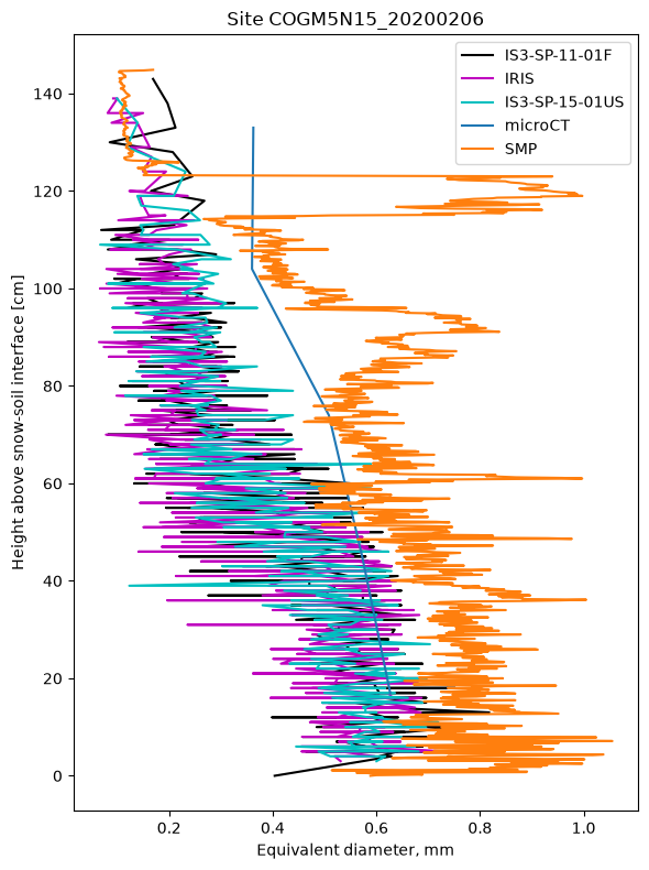
Wow, so the datasets are so very different, with the SMP being by far the most different. Comparing with Calonne et al., 2020 shows that the SMP is off in the same direction as diagnosed in that paper. Thus, the difference is most likely due to the difference in SMP instruments. Dr. Mel Sandells of Northumbria University has a github branch of the SMP software SnowMicropyn that has the newer fit relationship integrated in the software. It would be a nice project to loop in Mel’s branch with this notebook and see how well things compare to SnowEx data. I’d be happy to help anyone interested get rolling on that!
There’s also significant differences between the microCT and the two integrating spheres. This is science - sometimes when we start intercomparing these quantities, we do not get a perfect match. This would also be a fascinating thing to explore in a Hackweek project.
Some of the ways to could connect microstructure measurements to other quantities would be with the SWESARR radar data. Although the radar data does seem to have some orthorectification issues that haven’t been fully worked out, I can imagine these being worked around by careful choice of places you match up the microstructure to the radar. Note that places that are shallower tend to have larger Deq and vice versa, and the spatial variability in SSA was fairly low in general in Grand Mesa 2020, so looking at multiple SSA vs radar samples might not yield a great correlation.
One thing that could be of great value is to calibrate the SMP estimates of SSA to the integrating spheres. It might also be interesting to compare the data to hand hardness measured in the snowpit, and to traditional hand lens measurements.
Acknowledgments
Contributions from: Micah Johnson, Mike Durand, HP Marshall, Tate Meehan, Megan Mason, Scott Henderson. This relies heavily on the snowexsqul database and example scripts created by Micah Johnson.
- Dozier, J., Green, R. O., Nolin, A. W., & Painter, T. H. (2009). Interpretation of snow properties from imaging spectrometry. Remote Sensing of Environment, 113, S25 S37. 10.1016/j.rse.2007.07.029
- Ulaby, F. (2014). Microwave radar and radiometric remote sensing. University of Michigan Press.
- Mätzler, C. (2002). Relation between grain-size and correlation length of snow. Journal of Glaciology, 48(162), 461–466. 10.3189/172756502781831287
- Matzl, M., & Schneebeli, M. (2010). Stereological measurement of the specific surface area of seasonal snow types: Comparison to other methods, and implications for mm-scale vertical profiling. Cold Regions Science and Technology, 64(1), 1–8. 10.1016/j.coldregions.2010.06.006
- Löwe, H., Spiegel, J. K., & Schneebeli, M. (2011). Interfacial and structural relaxations of snow under isothermal conditions. Journal of Glaciology, 57(203), 499 510.
- Grenfell, T. C., & Warren, S. G. (1999). Representation of a nonspherical ice particle by a collection of independent spheres for scattering and absorption of radiation. Journal of Geophysical Research - Atmospheres, 104(D24), 31697 31709. doi:10.1029/1999JD900496
- HEGGLI, M., CHLE, B., Matzl, M., PINZER, B., RICHE, F., STEINER, S., STEINFELD, D., & Schneebeli, M. (2011). Measuring snow in 3-D using X-ray tomography: assessment of visualization techniques. Annals of Glaciology, 52(58), 231.
- Gallet, J. C., Domine, F., Zender, C. S., & Picard, G. (2009). Measurement of the specific surface area of snow using infrared reflectance in an integrating sphere at 1310 and 1550 nm. The Cryosphere, 3, 167 182.
- Leppänen, L., & Kontu, A. (2018). Analysis of QualitySpec Trek Reflectance from Vertical Profiles of Taiga Snowpack. Geosciences, 8(11), 404. 10.3390/geosciences8110404
- Montpetit, B., Royer, A., Langlois, A., Cliche, P., Roy, A., Champollion, N., Picard, G., Domine, F., & Obbard, R. (2012). New shortwave infrared albedo measurements for snow specific surface area retrieval. Journal of Glaciology, 58(211), 941 952. 10.3189/2012jog11j248
- Löwe, H., & Herwijnen, A. van. (2012). A Poisson shot noise model for micro-penetration of snow. Cold Regions Science and Technology, 70, 62–70. 10.1016/j.coldregions.2011.09.001
- Proksch, M., Löwe, H., & Schneebeli, M. (2015). Density, specific surface area, and correlation length of snow measured by high‐resolution penetrometry. Journal of Geophysical Research: Earth Surface, 120(2), 346–362. 10.1002/2014jf003266
- Calonne, N., Richter, B., Löwe, H., Cetti, C., Schure, J. ter, Herwijnen, A. V., Fierz, C., Jaggi, M., & Schneebeli, M. (2020). The RHOSSA campaign: multi-resolution monitoring of the seasonal evolution of the structure and mechanical stability of an alpine snowpack. The Cryosphere, 14(6), 1829–1848. 10.5194/tc-14-1829-2020