UAVSAR

Developers:

Jack Tarricone, University of Nevada, Reno
Zach Keskinen, Boise State University

Other contributors:

Ross Palomaki, Montana State University
Naheem Adebisi, Boise State University

What is UAVSAR?¶

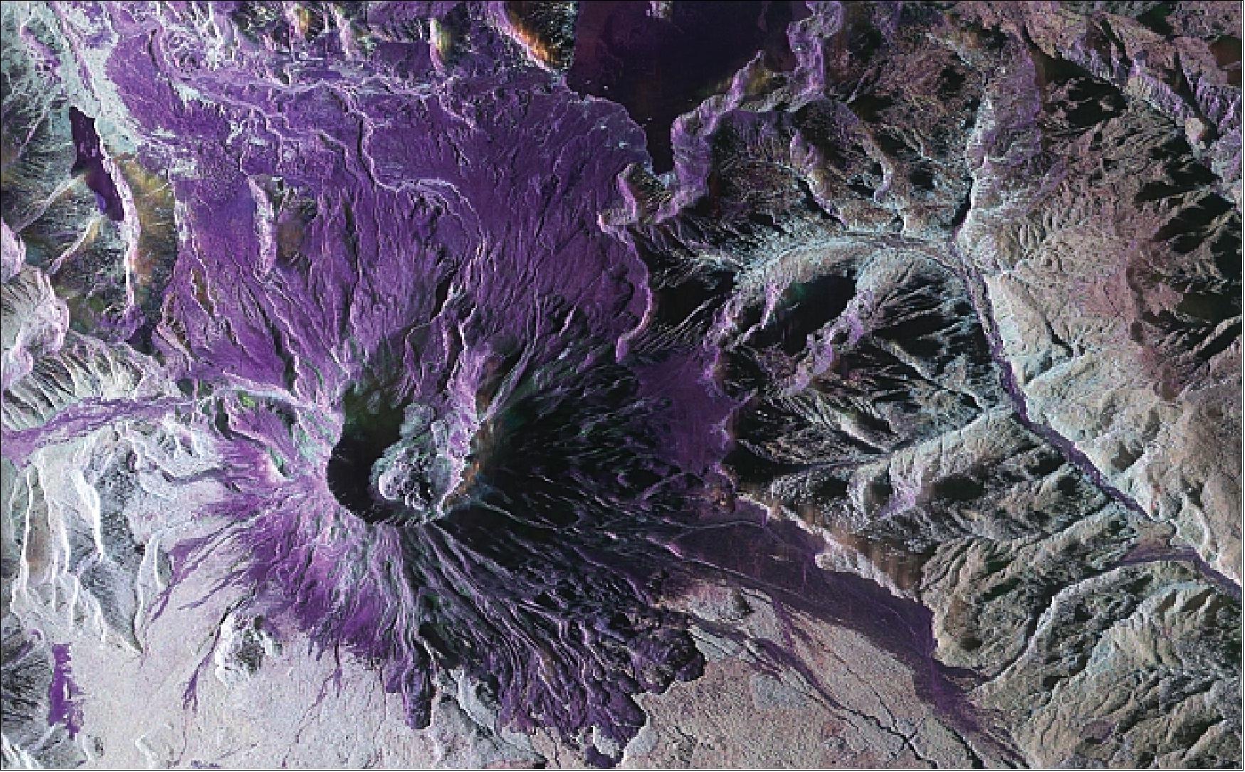
UAVSAR is a low frequency plane-based synthetic aperture radar. UAVSAR stands for “Uninhabited Aerial Vehicle Synthetic Aperture Radar”. It captures imagery using a L-band radar. This low frequency means it can penetrate into and through clouds, vegetation, and snow.

frequency (cm)	resolution (rng x azi m)	Swath Width (km)	Polarizations	Launch date
L-band 23	1.8 x 5.5	16	VV, VH, HV, HH	2007

NASA SnowEx 2020 and 2021 UAVSAR Campaigns¶

During the winter of 2020 and 2021, NASA conducted an L-band InSAR timeseries across the Western US with the goal of tracking changes in SWE. Field teams in 13 different locations in 2020, and in 6 locations in 2021, deployed on the date of the flight to perform calibration and validation observations.

The site locations from the above map along with the UAVSAR defined campaign name and currently processed pairs of InSAR images for each site. Note that the image pair count may contain multiple versions of the same image and may increase as more pairs of images are processed by JPL. Also note that the Lowman campaign name is the wrong state when searching.

Site Location	Campaign Name	Image Pairs
Grand Mesa	Grand Mesa, CO	13
Boise River Basin	Lowman, CO	17
Frazier Experimental Forest	Fraser, CO	16
Senator Beck Basin	Ironton, CO	9
East River	Peeler Peak, CO	4
Cameron Pass	Rocky Mountains NP, CO	15
Reynold Creek	Silver City, ID	1
Central Agricultral Research Center	Utica, MT	2
Little Cottonwoody Canyon	Salt Lake City, UT	21
Jemez River	Los Alamos, NM	3
American River Basin	Eldorado National Forest, CA	4
Sagehen Creek	Donner Memorial State Park, CA	4
Lakes Basin	Sierra National Forest, CA	3

Why would I use UAVSAR?¶

UAVSAR works with low frequency radar waves. These low frequencies (< 3 GHz) can penetrate clouds and maintain coherence (a measure of radar image quality) over long periods. For these reasons, time series was captured over 13 sites as part of the winter of 2019-2020 and 2020-2021 for snow applications. Additionally the UAVSAR is awesome!

Accessing UAVSAR Images¶

UAVSAR imagery can be downloaded from both the JPL and Alaska Satellite Facility. However both provide the imagery in a binary format that is not readily usable or readable by GIS software or python libraries.

Data Download and Conversion with `uavsar_pytools`¶

uavsar_pytools (Github) is a Python package developed out of work started at SnowEx Hackweek 2021. It nativiely downloads, formats, and converts this data in analysis ready rasters projected in WSG-84 Lat/Lon (EPSG:4326. The data traditionally comes in a binary format, which is not injestible by traditional geospatial analysis software (Python, R, QGIS, ArcGIS). It can download and convert either individual images - UavsarScene or entire collections of images - UavsarCollection.

Netrc Authorization¶

In order to download uavsar images you will need a netrc file that contains your earthdata username and password. If you need to register for a NASA earthdata account use this link. A netrc file is a hidden file, it won’t appear in the your file explorer, that is in your home directory and that programs can access to get the appropriate usernames and passwords. While you’ll have already done this for the Hackweek virtual machines, uavsar_pytools has a tool to create this netrc file on a local computer. You only need to create this file once and then it should be permanently stored on your computer.

# ## Creating .netrc file with Earthdata login information
# from uavsar_pytools.uavsar_tools import create_netrc

# # This will prompt you for your username and password and save this
# # information into a .netrc file in your home directory. You only need to run
# # this command once per computer. Then it will be saved.
# create_netrc()

Downloading and converting a single UAVSAR interferogram scene¶

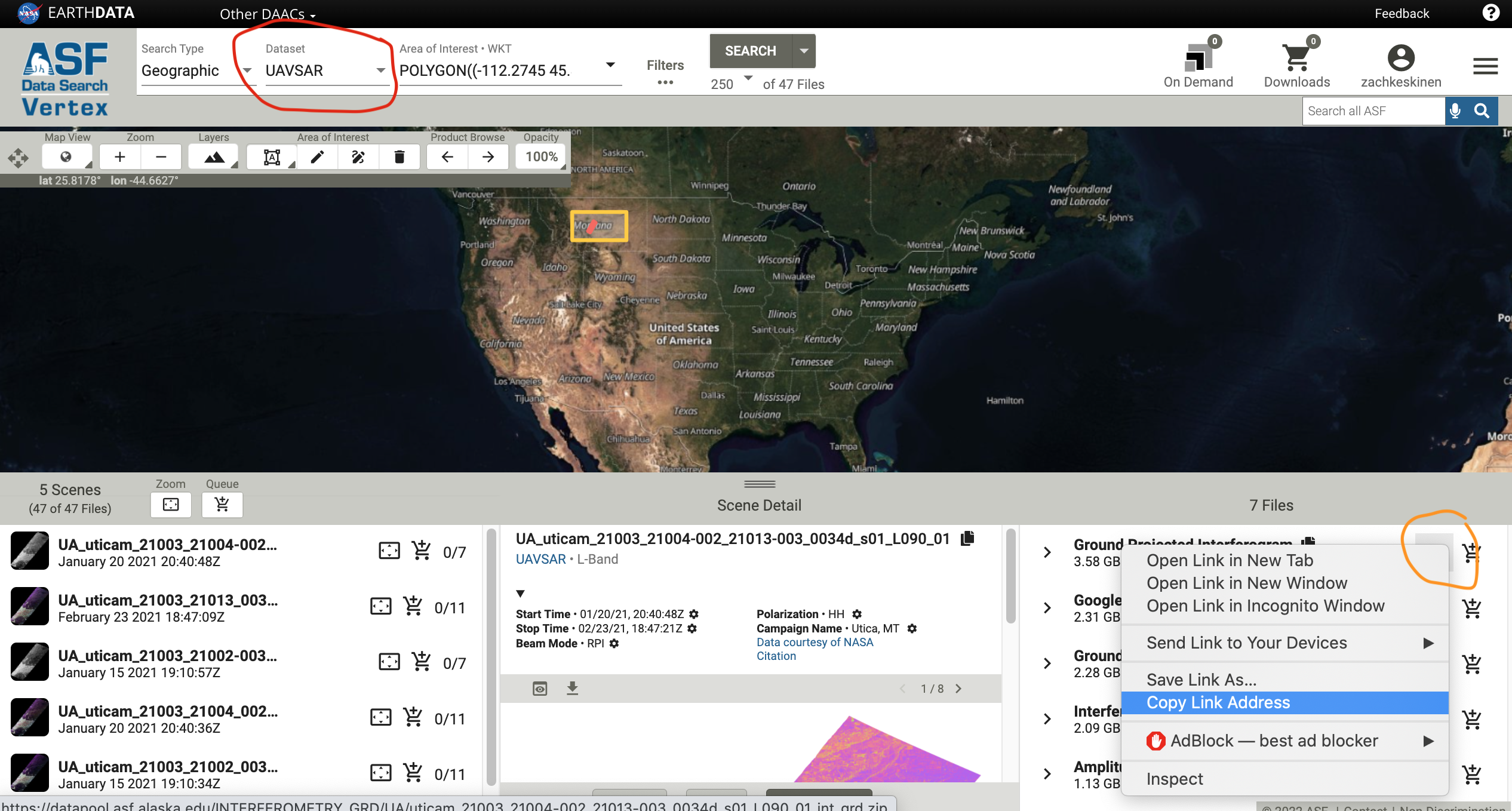
You can find urls for UAVSAR images at the ASF vertex website. Make sure to change the platform to UAVSAR and you may also want to filter to ground projected interferograms.

try:
    from uavsar_pytools import UavsarScene
except ModuleNotFoundError:
    print('Install uavsar_pytools with `pip install uavsar_pytools`')

## This is the directory you want to download and convert the images in.
work_dir = '/tmp/uavsar_data'

## This is a url you want to download. Can be obtained from vertex
url = 'https://datapool.asf.alaska.edu/INTERFEROMETRY_GRD/UA/\
lowman_23205_21009-004_21012-000_0007d_s01_L090_01_int_grd.zip'

## clean = True will delete the binary and zip files leaving only the tiffs
scene = UavsarScene(url = url, work_dir=work_dir, clean= True)

## After running url_to_tiffs() you will download the zip file, unzip the binary 
## files, and convert them to geotiffs in the directory with the scene name in
## the work directory. It also generate a .csv pandas dictionary of metadata.
# scene.url_to_tiffs()

/home/runner/micromamba/envs/snow-observations-cookbook/lib/python3.14/site-packages/tqdm/auto.py:21: TqdmWarning: IProgress not found. Please update jupyter and ipywidgets. See https://ipywidgets.readthedocs.io/en/stable/user_install.html
  from .autonotebook import tqdm as notebook_tqdm

Downloading and converting a full UAVSAR collection¶

If you want to download and convert an entire Uavsar collection for a larger analysis you can use UavsarCollection. The collection names for the SnowEx campaign are listed in the table in the introduction. The UavsarCollection can download either InSAR pairs and PolSAR images.

from uavsar_pytools import UavsarCollection
## Collection name, the SnowEx Collection names are listed above. These are case 
## and space sensitive.
collection_name = 'Grand Mesa, CO'

## Directory to save collection into. This will be filled with directory with 
## scene names and tiffs inside of them.
out_dir = '/tmp/collection_ex/'

## This is optional, but you will generally want to at least limit the date
## range between 2019 and today.
date_range = ('2019-11-01', 'today')

# Keywords: to download incidence angles with each image use `inc = True`
# For only certain pols use `pols = ['VV','HV']`

collection = UavsarCollection(collection = collection_name, work_dir = out_dir, dates = date_range)

## You can use this to check how many image pairs have at least one image in
## the date range.

#collection.find_urls()

## When you are ready to download all the images run:

# collection.collection_to_tiffs()

## This will take a long time and a lot of space, ~1-5 gB and 10 minutes per 
## image pair depending on which scene, so run it if you have the space and time.

UAVSAR Data Products¶

UAVSAR has a variety of different type of images:

Repeat Pass Interferometric images contain:

UAVSAR repeat pass interferometry uses two images of the same place but separated in time. Phase changes between the two aquistions are calculated, creating a wrapped interferogram. These phase changes are due to either the wave traveling a longer distance (ground movement or refraction) or change wave speeds (atmospheric water vapor and snow).

GRD files (.grd): products projected to the ground in geographic coordinates (latitude, longitude) Finally all images can be in radar slant range or projected into WGS84. Images that have already been projected to ground range will have the extension .grd appended to their file type extension.

For instance a image of unwrapped phase that has not been georefenced would end with .unw, while one that was georeferenced would end with .unw.grd. You will generally want to use .grd files for most analysis.

Polarimetric PolSAR images contain:

ANN file (.ann): a text annotation file with metadata
Polsar file (HHVV.grd): all the rest of the files will be a pair of polarizations pushed together

Polsar files have a pair of polarizations (VV, VH, HV, HH) combined in their file name. These files are the phase difference between polarization XX and polarization YY. For instance HHHV is the phase difference between HH and HV polarizations. HVVV is the phase difference between HV and VV and so one. There are 6 of these pairs since order is irrelevant. These 6 images are combined to calculate various metrics that tell you about the types of scattering occurring.

Import Libraries¶

try:
    from uavsar_pytools import UavsarScene
    from uavsar_pytools.snow_depth_inversion import depth_from_phase, phase_from_depth
except ModuleNotFoundError:
    print('Install uavsar_pytools with `pip install uavsar_pytools`')

import os
from os.path import join, basename
import matplotlib.pyplot as plt
from glob import glob
import numpy as np
import pandas as pd
import seaborn as sns
import holoviews as hv
import rioxarray as rxa
import rasterio as rio
from bokeh.plotting import show
import datashader as ds
from datashader.mpl_ext import dsshow
hv.extension('bokeh', logo=False)
import contextily as cx
from datetime import date
from shapely.geometry import box
import requests
%config InlineBackend.figure_format='retina'

# Database 
from snowexsql.lambda_client import SnowExLambdaClient

import warnings
warnings.filterwarnings('ignore', category=UserWarning, module='rasterio')
warnings.filterwarnings('ignore', category=UserWarning, module='rioxarray')
warnings.filterwarnings('ignore', category=FutureWarning)
import logging
logging.getLogger('rasterio._env').setLevel(logging.ERROR)
logging.getLogger('rasterio._filepath').setLevel(logging.ERROR)
os.environ['CPL_CURL_VERBOSE'] = 'NO'
os.environ['CPL_DEBUG'] = 'OFF'  # Suppress GDAL debug messages
os.environ['GDAL_HTTP_UNSAFESSL'] = 'YES'  # Optional: if SSL issues occur
os.environ['GDAL_DISABLE_READDIR_ON_OPEN'] = 'EMPTY_DIR'  # Prevent mask file lookups

def plot_rgb_image(rgb_array, figsize=(15, 15), title="RGB Image", stretch=True, ax=None):
    """Plot RGB image from stacked array"""
    if ax is None:
        fig, ax = plt.subplots(figsize=figsize)
    else:
        fig = ax.get_figure()
    
    # Get RGB bands (expecting shape: bands, height, width)
    rgb_display = np.stack([rgb_array[0], rgb_array[1], rgb_array[2]], axis=-1)
    
    if stretch:
        # Apply percentile stretch for better visualization
        p2, p98 = np.percentile(rgb_display[~np.isnan(rgb_display)], (2, 98))
        rgb_display = np.clip((rgb_display - p2) / (p98 - p2), 0, 1)
    
    ax.imshow(rgb_display)
    ax.set_title(title, fontsize=16)
    ax.axis('off')
    
    return fig, ax

Interferometric Imagery¶

In this section we’ll be plotting and comparing dirrerent types of SAR and InSAR data with optical imagery and a digital elevation model. For this example we’ll be taking a subet of the Lowman flight (Boise, ID) line encompassing Banner Summit.

Access Tutorial Data from S3¶

The tutorial data is hosted on AWS S3 and can be accessed directly without downloading. The data will be streamed as needed using rioxarray.

# S3 base URL for tutorial data
S3_BASE_URL = "https://snowex-tutorials.s3.us-west-2.amazonaws.com/uavsar/"

Load in Rasters¶

Here we’ll load our rasters into the environemtns using rioxarray or rxa, we will then convert to a np.array to be able to use matplotlib.pyplot or plt for plotting

Optical Data¶

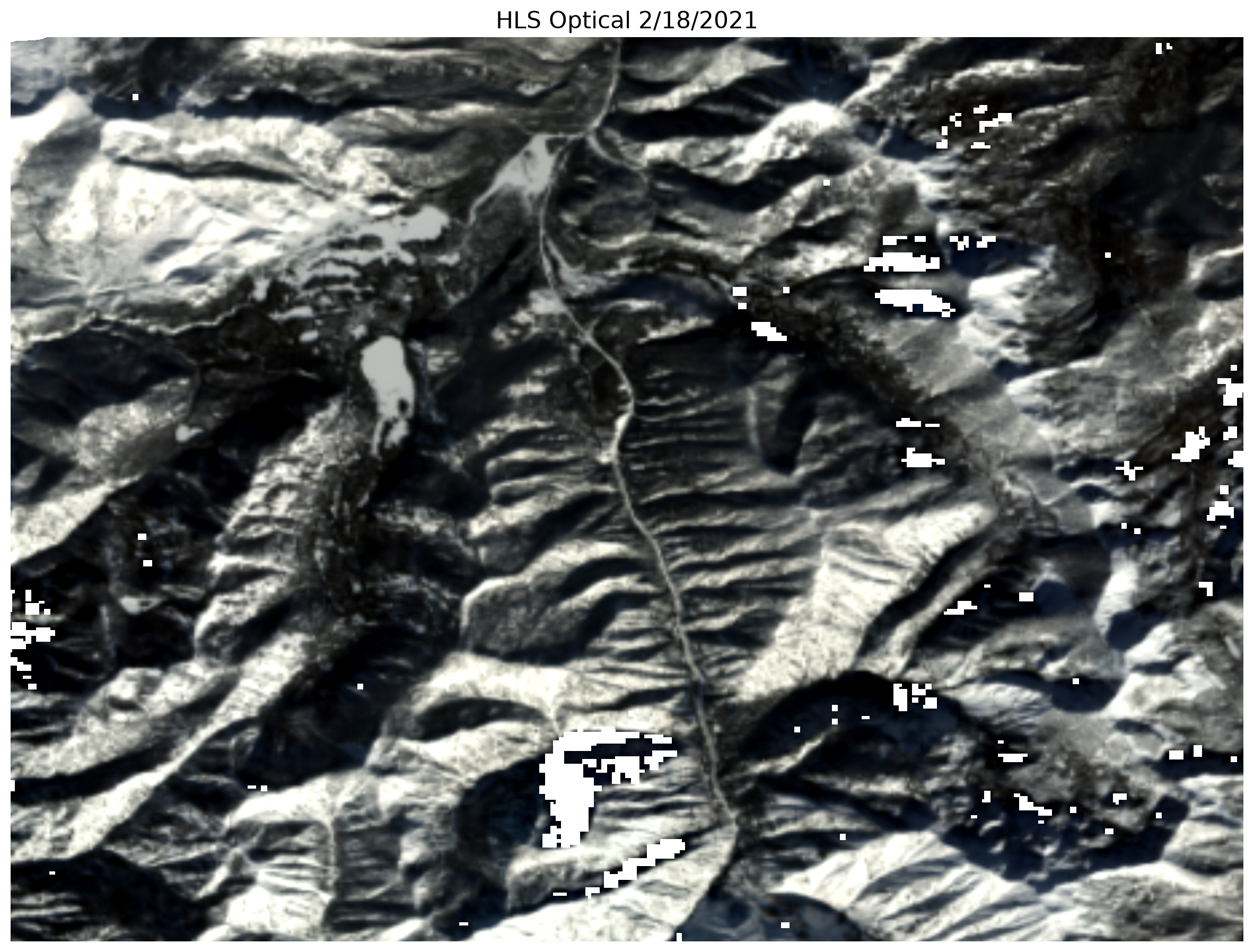
We will be using Haromized Landsat Sentinel (HLS) dataset from January 13th, 2021. This date was selected because it is mostly cloud free, which is uncommon in mountain environments during the winter.

# Define S3 URLs for the three RGB bands and stack them in memory
red_path = S3_BASE_URL + 'lowman_red.tif'
green_path = S3_BASE_URL + 'lowman_green.tif'
blue_path = S3_BASE_URL + 'lowman_blue.tif'

# Load and stack RGB bands directly from S3 (no local files needed)
import xarray as xr
red = rxa.open_rasterio(red_path)
green = rxa.open_rasterio(green_path)
blue = rxa.open_rasterio(blue_path)

# Stack the bands into a single array
rgb = xr.concat([red, green, blue], dim='band')
rgb['band'] = [1, 2, 3]  # Label bands as 1, 2, 3

What do we see in this image? Any notable features?¶

# plot rgb image

plot_rgb_image(rgb.values, figsize=(15, 15), title="HLS Optical 2/18/2021", stretch=True)
plt.show()

InSAR and SAR Data¶

Here we’ll be using five different data products related to InSAR and SAR: unwrapped phase (unw), coherence (cor), amplitude (amp), elevation (dem), and incidence angle (inc).

# Open rasters directly from S3 and inspect metadata using xarray
unw_rast  = rxa.open_rasterio(S3_BASE_URL + 'lowman_unw.tif')
unw = unw_rast[0].values # np.array for plotting
    
# coherence
cor_rast  = rxa.open_rasterio(S3_BASE_URL + 'lowman_cor.tif')
cor = cor_rast[0].values

# amplitude
amp_rast  = rxa.open_rasterio(S3_BASE_URL + 'lowman_amb_db.tif')
amp = amp_rast[0].values # np.array for plotting

# dem
dem_rast  = rxa.open_rasterio(S3_BASE_URL + 'lowman_dem.tif')
dem = dem_rast[0].values

# incidence angle
inc_rast  = rxa.open_rasterio(S3_BASE_URL + 'lowman_inc_deg.tif')
inc = inc_rast[0].values # np.array for plotting

# plot unwrapped phase

plt.rcParams.update({'font.size': 12}) # increase plot font size for larger plot
fig, ax = plt.subplots(figsize=(15, 15))

ax.set_title("UNW (radians)", fontsize= 20) #title and font size
img = ax.imshow(unw, interpolation = 'nearest', cmap = 'viridis', vmin = -3, vmax = 2)

# add legend
colorbar = fig.colorbar(img, ax=ax, fraction=0.03, pad=0.04) # add color bar
plt.show()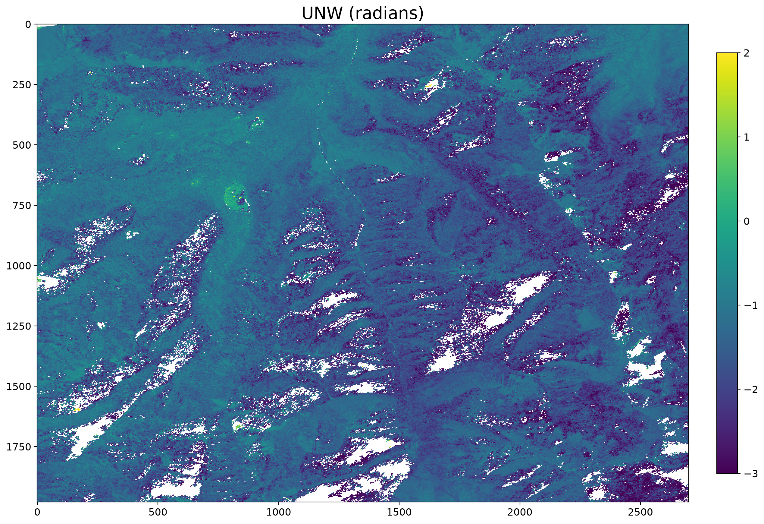

# plot coherence

plt.rcParams.update({'font.size': 12}) # increase plot font size for larger plot
fig, ax = plt.subplots(figsize=(15, 15))

ax.set_title("Coherence", fontsize= 20) #title and font size
img = ax.imshow(cor, cmap = 'magma', vmin = 0, vmax = 1)

# add legend
colorbar = fig.colorbar(img, ax=ax, fraction=0.03, pad=0.04) # add color bar
plt.show()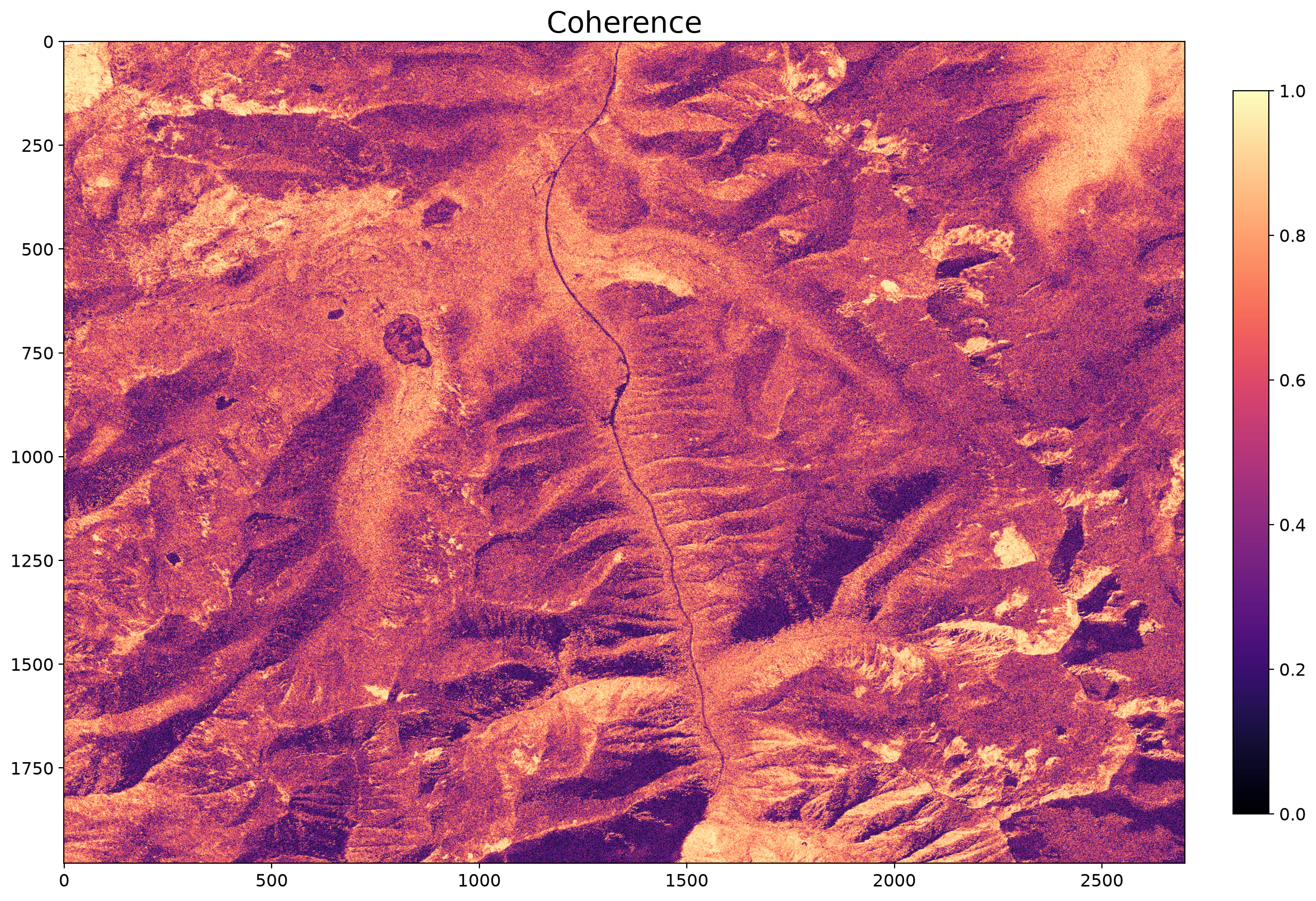

# plot amplitude

plt.rcParams.update({'font.size': 12}) # increase plot font size for larger plot
fig, ax = plt.subplots(figsize=(15, 15))

ax.set_title("Amplitude (dB)", fontsize= 20) #title and font size
img = ax.imshow(amp, cmap = 'Greys_r', vmin = -20, vmax = 0)

# add legend
colorbar = fig.colorbar(img, ax=ax, fraction=0.03, pad=0.04) # add color bar
plt.show()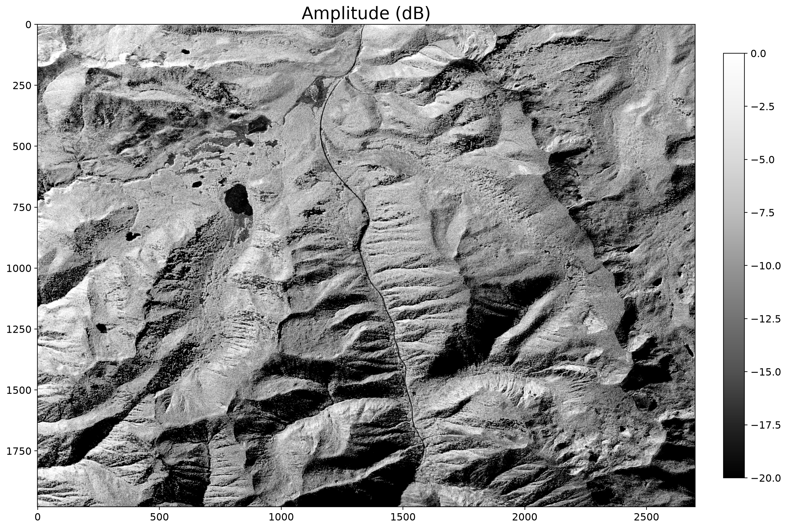

# plot dem

plt.rcParams.update({'font.size': 12}) # increase plot font size for larger plot
fig, ax = plt.subplots(figsize=(15, 15))

ax.set_title("Elevation (m)", fontsize= 20) #title and font size
img = ax.imshow(dem, cmap = 'terrain', vmin = 1800, vmax = 2800)

# add legend
colorbar = fig.colorbar(img, ax=ax, fraction=0.03, pad=0.04) # add color bar
plt.show()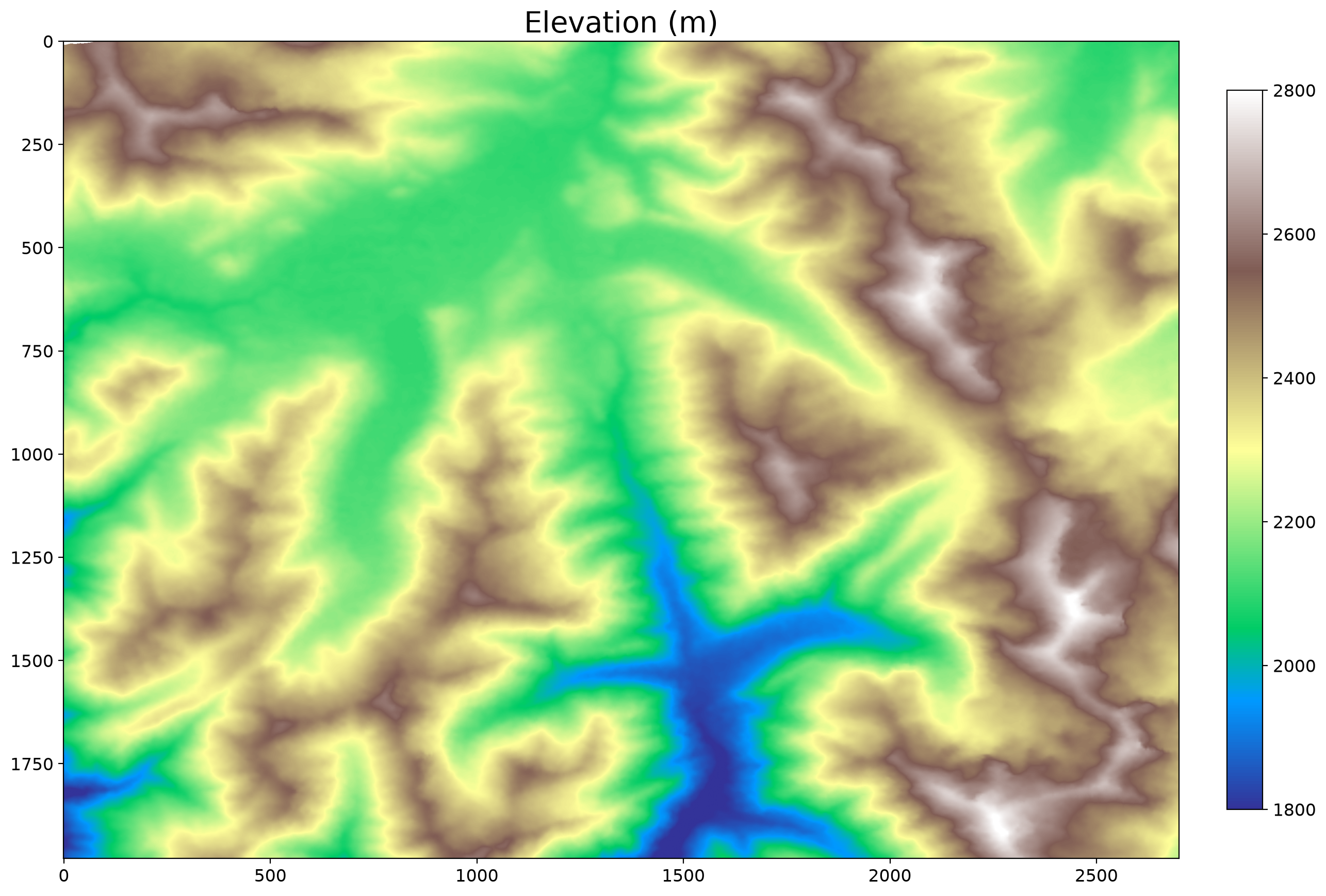

# plot incidence angle

plt.rcParams.update({'font.size': 12}) # increase plot font size for larger plot
fig, ax = plt.subplots(figsize=(15, 15))

ax.set_title("Incidence Angle (deg)", fontsize= 20) #title and font size
img = ax.imshow(inc, cmap = 'Spectral_r', vmin = 20, vmax = 90)

# add legend
colorbar = fig.colorbar(img, ax=ax, fraction=0.03, pad=0.04) # add color bar
plt.show()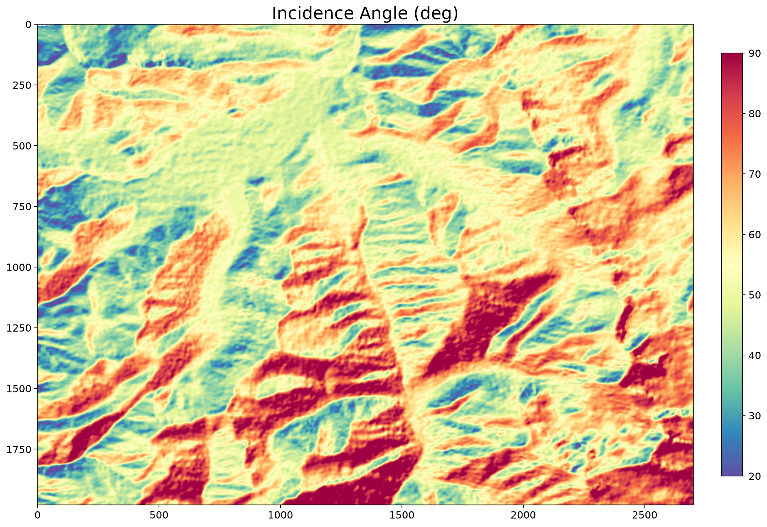

Comparison Plot¶

# plot all InSAR products
fig = plt.figure(figsize=(30,19))

ax = fig.add_subplot(1,3,1)
cax=ax.imshow(unw, cmap='viridis', interpolation = 'nearest', vmin = -3, vmax = 2)
ax.set_title("UNW (radians)")
cbar = fig.colorbar(cax, ticks=[-3,0,2],orientation='horizontal', fraction=0.03, pad=0.04)
cbar.ax.set_xticklabels([-3,0,2])

ax = fig.add_subplot(1,3,2)
cax = ax.imshow(cor, cmap = 'magma', vmin = 0, vmax = 1)
ax.set_title("Coherence")
cbar = fig.colorbar(cax, ticks=[0,.5,1], orientation='horizontal',fraction=0.03, pad=0.04)


ax = fig.add_subplot(1,3,3)
cax = ax.imshow(amp, cmap = 'Greys_r', vmin = -20, vmax = 0)
ax.set_title("Amplitude (dB)")
cbar = fig.colorbar(cax, ticks=[-20,-10,0], orientation='horizontal',fraction=0.03, pad=0.04)
cbar.ax.set_xticklabels([-20,-10,0])

ax = fig.add_subplot(2,3,1)
cax = ax.imshow(inc, cmap = 'Spectral_r', vmin = 20, vmax = 90)
ax.set_title("Incidence Angle (deg)")
cbar = fig.colorbar(cax, ticks=[20,90], orientation='horizontal', pad=0.07)
cbar.ax.set_xticklabels([20,90])

ax = fig.add_subplot(2,3,2)
cax = ax.imshow(dem, cmap = 'terrain', vmin = 1800, vmax = 2800)
ax.set_title("Elevation (m)")
cbar = fig.colorbar(cax, ticks=[1800,2800], orientation='horizontal', pad=0.07)
cbar.ax.set_xticklabels([1800,2800])

done = None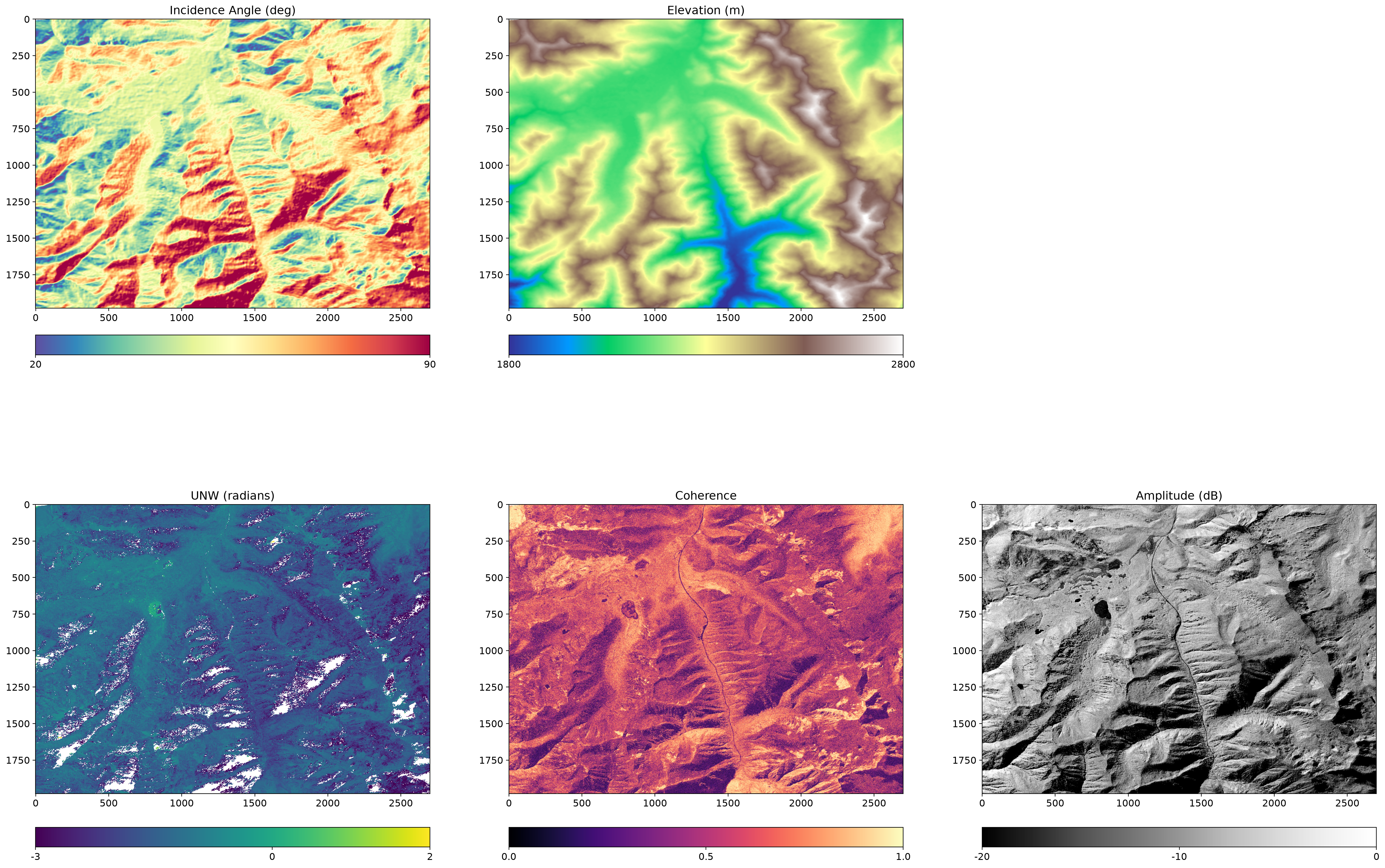

plot_rgb_image(rgb.values, figsize=(7, 7), title="HLS Optical 2/18/2021", stretch=True)
plt.show()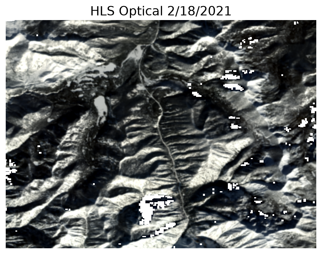

What are some notable similarities between images? Differences?¶

In the next section we’ll go into more detail about the features that impact coherence, phase, and how they’re related

Sagehen Creek Example¶

# Load Sagehen Creek data directly from S3
sage_files = ['cor.tif', 'hgt.tif', 'unw.tif']
imgs = {}
for filename in sage_files:
    name = filename.split('.')[0]
    s3_path = S3_BASE_URL + 'sage/' + filename
    imgs[name] = rxa.open_rasterio(s3_path, parse_coordinates=True, default_name=name)

What topographic features seem to impact coherence?¶

Take a moment to chat with the people around you about this. Some features to get you thinking:

lakes
aspect (south vs north, east vs west)
elevation
trees
roads
others?

tiles = hv.element.tiles.EsriUSATopo().opts()
cor = hv.Image(hv.Dataset(imgs['cor'], kdims=['x','y'])).opts(cmap = 'gray', colorbar=True, xaxis = None, yaxis = None, title = 'Coherence')
hgt = hv.Image(hv.Dataset(imgs['hgt'], kdims=['x','y'])).opts(cmap = 'terrain', colorbar=True, xaxis = None, yaxis = None, title= 'DEM', alpha = 0.4)
hgt_trans = hv.Image(hv.Dataset(imgs['hgt'][0,::100,::100], kdims=['x','y'])).opts(alpha = 0, xaxis = None, yaxis = None, title = 'Topo')
cor_tile = tiles  * cor
hgt_tile = tiles  * hgt
imagery = hv.element.tiles.EsriImagery()  * hgt_trans

hv.Layout([cor_tile, hgt_tile, imagery]).opts(width = 400, height = 900)

import seaborn as sns
xna = imgs['hgt'].data.ravel()
yna = imgs['cor'].data.ravel()
x = xna[(~np.isnan(xna)) & (~np.isnan(yna))][::100]
y = yna[(~np.isnan(xna)) & (~np.isnan(yna))][::100]

df = pd.DataFrame(dict(x=x, y=y))
df['x_cat'] = pd.qcut(df.x, q= 6, precision = 0)
f, ax = plt.subplots(figsize = (12,8))
sns.violinplot(y = df.y[::100], x = df.x_cat[::100], scale = 'count')
plt.xlabel('Elevation Bands (m)')
plt.ylabel('Coherence')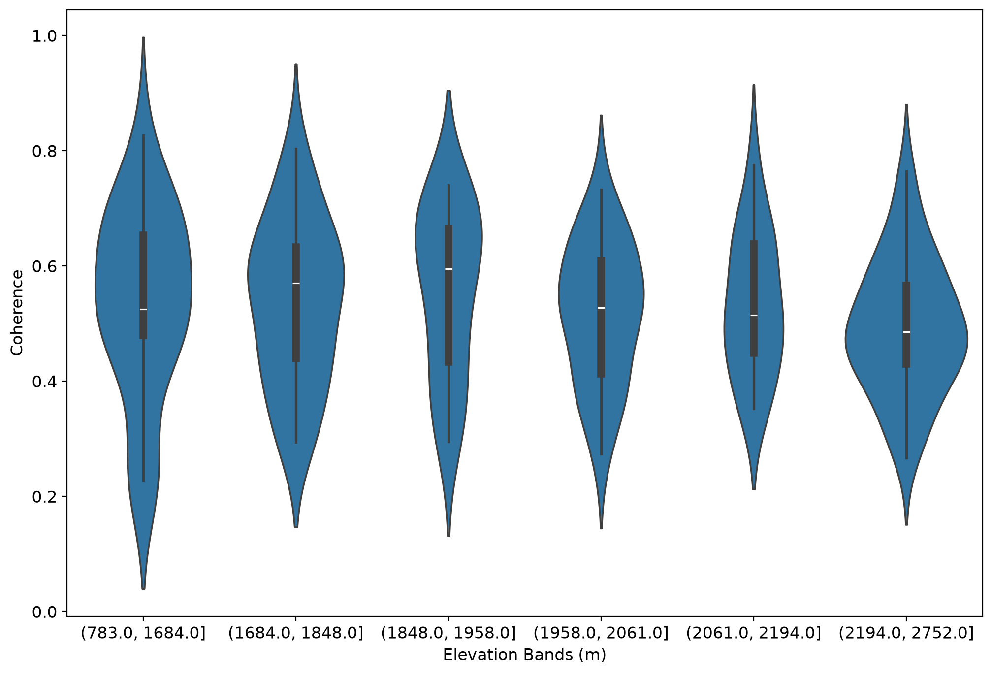

UNW vs. Coherence¶

tiles = hv.element.tiles.EsriUSATopo().opts()
cor = hv.Image(hv.Dataset(imgs['cor'], kdims=['x','y'])).opts(cmap = 'gray', colorbar=True, xaxis = None, yaxis = None, title = 'Coherence')
unw = hv.Image(hv.Dataset(imgs['unw'], kdims=['x','y'])).opts(cmap = 'magma', colorbar=True, xaxis = None, yaxis = None, title= 'Unwrapped Phase', clim = (0, 2*np.pi))
cor_tile = tiles  * cor
unw_tile = tiles  * unw

hv.Layout([cor_tile, unw_tile]).opts(width = 400, height = 900)

Why would I use UAVSAR for snow?¶

L-band SAR penetrates through the snowpack. However when it crosses into the snowpack from the air it refracts at an angle, similar to light entering water. This refraction leads to a phase shift relative to an image with no or less snow. Using this difference in phase between two images we can calculate the change in snow height between flights using:

\Delta d = - \frac{\Delta \phi \lambda}{4 \pi} \frac{1}{\cos^{ } \alpha - \sqrt{\epsilon_{s} - \sin^{2} \alpha}}

(1)

Where $\Delta$ d is the change in snow height, $\Delta \phi$ is the phase shift between two SAR images, $\lambda$ is the radar wavelength, $\alpha$ is the incidence angle, and $\epsilon_{s}$ is the dielectric constant of snow which is dependent on the density and liquid water content.

Set variables¶

# Mesa Lake Snotel Coordinates
snotel_coords = (-108.05, 39.05)

Phase Change between February 1st and 13th UAVSAR Image Pairs¶

You learned in the first section how to access and download UAVSAR imagery. For this section the data has already been downloaded, converted to GeoTiffs and cropped down to an area of interest that overlaps the main field sites of Grand Mesa. Lets take a look at the coherence and unwrapped phase between these two flights. If you don’t remember what these two represent check out the previous section of this tutorial.

# Create figures and subplots
fig, axes = plt.subplots(2, 1, figsize = (12,8))

# Select colormap for each image type
vis_dic = {'cor': 'Blues', 'unw':'magma'}

# Loop through coherence and unwrapped phase images
for i, type in enumerate(vis_dic.keys()):
    # select correct axis
    ax = axes[i]
    # open image directly from S3 with rioxarray
    img = rxa.open_rasterio(S3_BASE_URL + f'{type}.tif')
    # calculate visualization parameters
    vmin, vmax = img.quantile([0.1,0.9])
    # plot images
    img.plot(ax = ax, vmin = vmin, vmax = vmax, cmap = vis_dic[type], zorder = 1, alpha = 0.7)
    # zoom out a bit
    ax.set_xlim(-108.28,-108)
    ax.set_ylim(38.98, 39.08)
    # add topo basemap
    cx.add_basemap(ax, crs=img.rio.crs, alpha = 0.8, source = cx.providers.USGS.USTopo)
    # turn off labels
    ax.xaxis.label.set_visible(False)
    ax.yaxis.label.set_visible(False)
# set titles
axes[0].set_title('Coherence')
axes[1].set_title('Unwrapped Phase Change')

plt.show()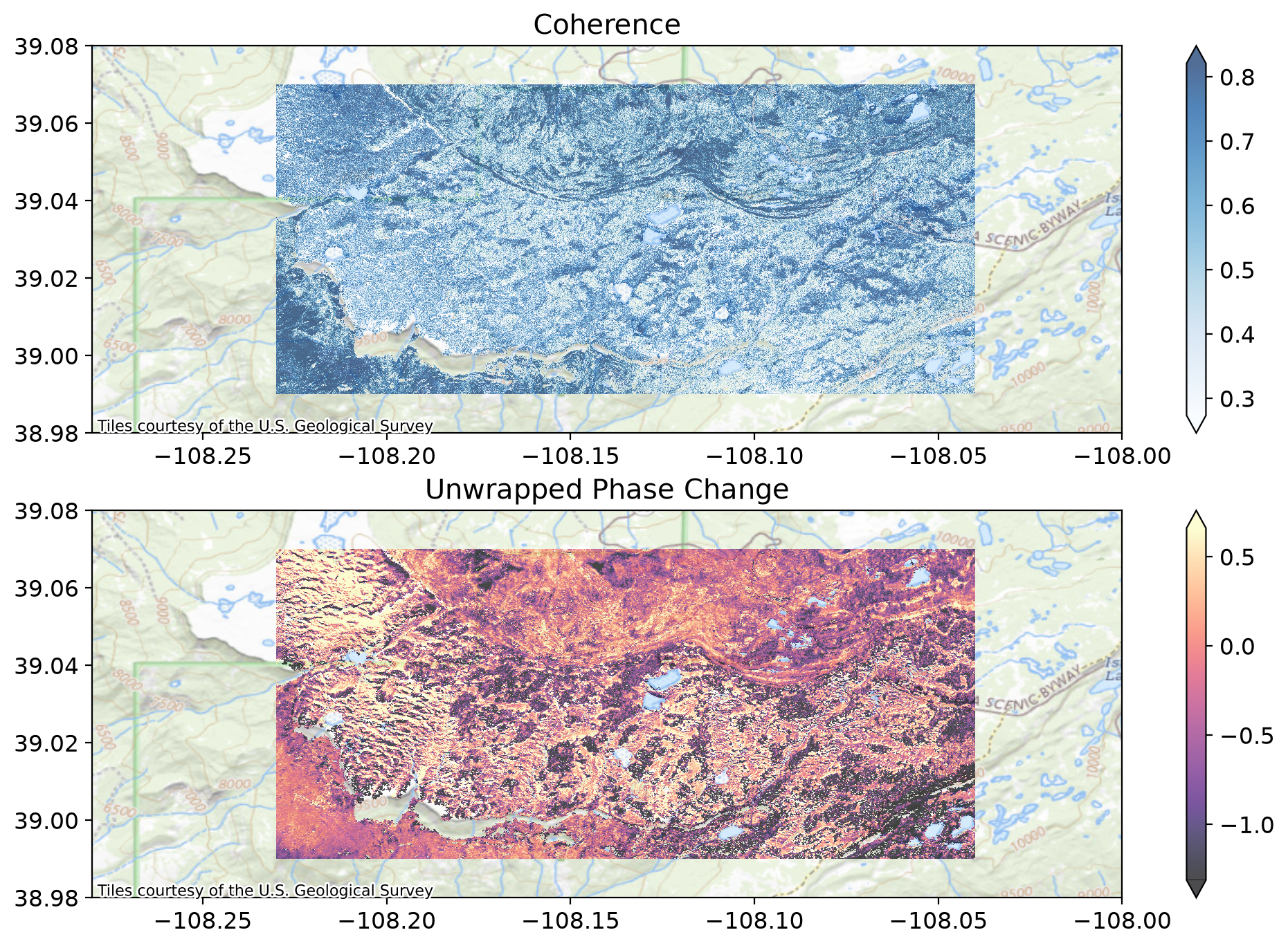

fig, ax = plt.subplots(figsize = (12,8))

# Plot the snotel location
ax.scatter(x = snotel_coords[0], y = snotel_coords[1], marker = 'x', color = 'black')

# Plot bounding box of uavsar - stream from S3
uavsar_bounds = rxa.open_rasterio(S3_BASE_URL + 'cor.tif').rio.bounds()
x,y = box(*uavsar_bounds).exterior.xy
ax.plot(x,y, color = 'blue')

# Set overview bounds
ax.set_xlim(-108.4,-107.75)
ax.set_ylim(38.75, 39.3)

# Add background map
cx.add_basemap(ax, crs='EPSG:4326', alpha = 0.8, source = cx.providers.USGS.USImageryTopo)
plt.title('Overview Map')
plt.show()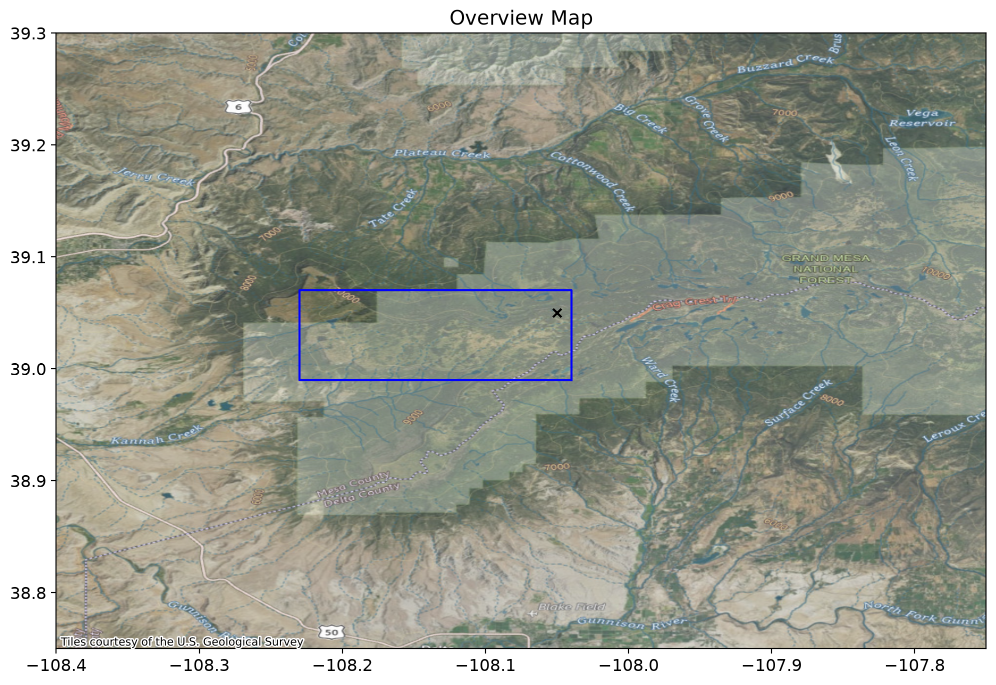

Using the SnowEx SQL Database to collect snow depth and lidar datasets¶

Lets explore how many overlapping depth observations we have between these two days. First we establish a connection to the database:

# Initialize client
client = SnowExLambdaClient()

# Get all measurement classes dynamically
classes = client.get_measurement_classes()
LayerMeasurements = classes['LayerMeasurements']
PointMeasurements = classes['PointMeasurements']

print("🔍 Testing Lambda connection...")
connection_test = client.test_connection()
print(f"✅ Connected: {connection_test.get('connected', False)}")
if connection_test.get('connected'):
    print(f"📊 Database: {connection_test.get('version', 'Unknown version')}")
else:
    print("❌ Connection failed")

🔍 Testing Lambda connection...

✅ Connected: True
📊 Database: PostgreSQL 16.10 on x86_64-conda-linux-gnu, compiled by x86_64-conda-linux-gnu-cc (conda-forge gcc 14.3.0-4) 14.3.0, 64-bit

Next, we will find snow depth data in a 1 day window around our two campaign dates of Feb 1 and Feb 12, 2020:

df_feb_1 = PointMeasurements.from_filter(
    campaign = 'Grand Mesa',
    type = 'depth',
    instrument='camera',
    date_greater_equal = date(2020, 1, 31),
    date_less_equal = date(2020, 2, 2),
)

df_feb_12 = PointMeasurements.from_filter(
    campaign = 'Grand Mesa',
    type = 'depth',
    instrument = 'camera',
    date_greater_equal = date(2020, 2, 11),
    date_less_equal = date(2020, 2, 13),
)

# Get depths that were captured on both days
df_both = df_feb_1.overlay(df_feb_12, how = 'intersection')

# Calculate the snow depth change for each point
df_both['sd_diff'] = df_both.value_2 - df_both.value_1

fig, ax = plt.subplots(figsize = (12,4))

# Plot depth measurements
df_both.plot(ax = ax, column = 'sd_diff', legend = True, legend_kwds = {'label': 'Snow Depth Change [cm]'}, cmap = 'magma')

# Plot the snotel location
snotel_coords = (-108.05, 39.05)
ax.scatter(x = snotel_coords[0], y = snotel_coords[1], marker = 'x', color = 'black')

# Plot bounding box of uavsar - stream from S3
img = rxa.open_rasterio(S3_BASE_URL + 'cor.tif')
uavsar_bounds = img.rio.bounds()
x,y = box(*uavsar_bounds).exterior.xy
ax.plot(x,y, color = 'blue')

# Set same bounds as uavsar image plot
ax.set_xlim(-108.28,-108)
ax.set_ylim(38.98, 39.08)

# Add background map
cx.add_basemap(ax, crs=img.rio.crs, alpha = 0.8, source = cx.providers.USGS.USImageryTopo)
plt.title('Database Snow Depth Measurements')
plt.show()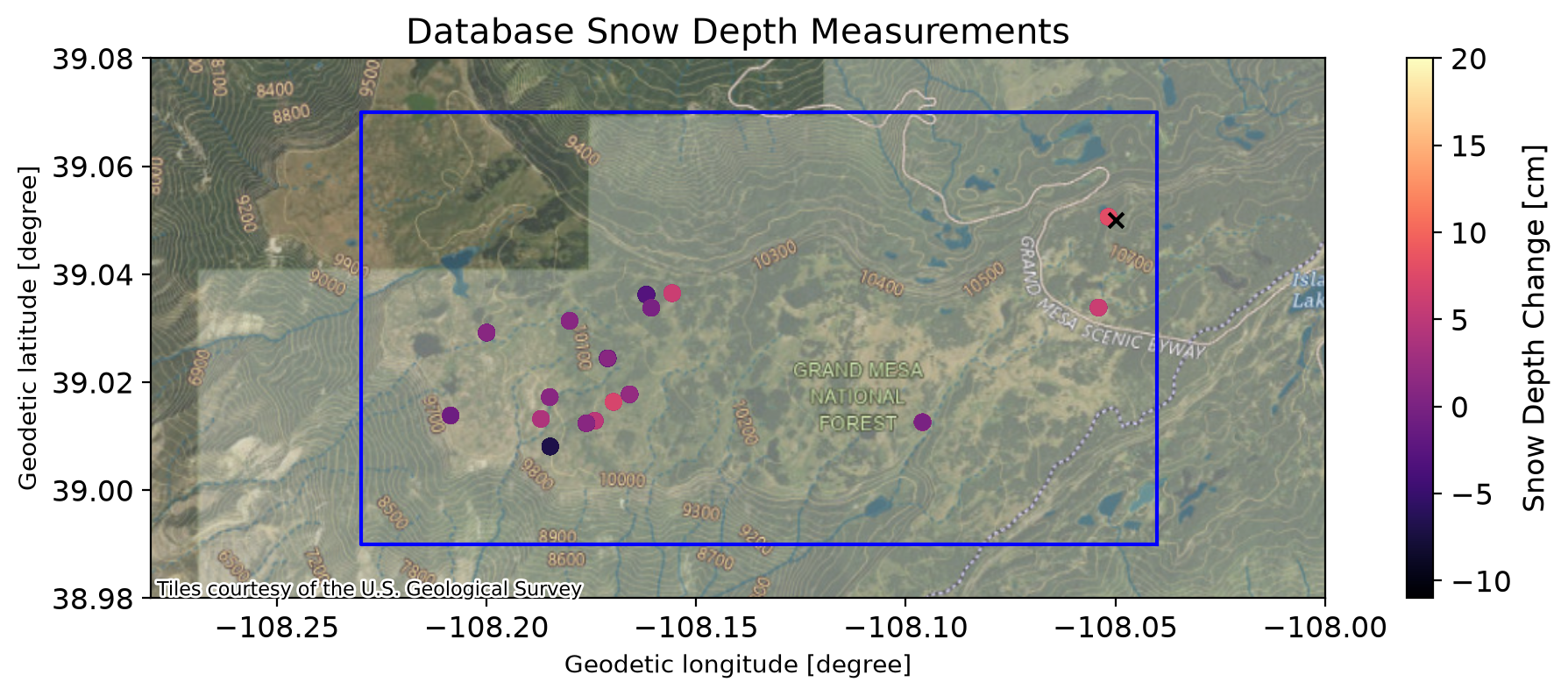

Getting the remaining parameters¶

Incidence Angle¶

We can recall the formula to calculate snow depth change from incidence angle, phase change, and the snow permittivity.

\Delta d = - \frac{\Delta \phi \lambda}{4 \pi} \frac{1}{\cos^{ } \alpha - \sqrt{\epsilon_{s} - \sin^{2} \alpha}}

(2)

We have two of these variables already: incidence angle and phase change.

# Create figures and subplots
fig, axes = plt.subplots(2, 1, figsize = (12,8))

# Select colormap for each image type
vis_dic = {'inc': 'Greys', 'unw':'magma'}

# Loop through each image type
for i, type in enumerate(vis_dic.keys()):
    ax = axes[i]
    # Open image directly from S3 with rioxarray
    img = rxa.open_rasterio(S3_BASE_URL + f'{type}.tif')
    # convert incidence angle from radians to degrees
    if type == 'inc':
        img = np.rad2deg(img)
    # this is a great convenience feature to calculate good visualization levels
    vmin, vmax = img.quantile([0.1,0.9])
    # plot the image
    im = img.plot(ax = ax, vmin = vmin, vmax = vmax, cmap = vis_dic[type], zorder = 1, alpha = 0.7)
    # Zoom out a big
    ax.set_xlim(-108.28,-108)
    ax.set_ylim(38.98, 39.08)
    # Add a topo basemap
    cx.add_basemap(ax, crs=img.rio.crs, alpha = 0.8, source = cx.providers.USGS.USTopo)
    # Remove unnecessary 'x' 'y' labels
    ax.xaxis.label.set_visible(False)
    ax.yaxis.label.set_visible(False)

# Add titles
axes[0].set_title('Incidence Angle')
axes[1].set_title('Unwrapped Phase Change')
plt.show()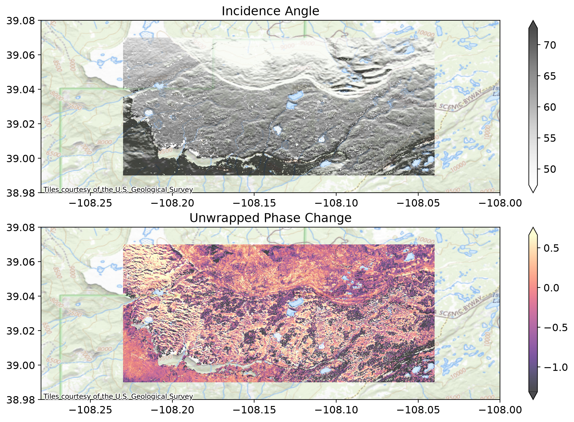

Getting Permittivity¶

We have two ways of getting the $e_{s}$ , or the real part of the snow’s dielectric permittivity. One is by estimating from the snow density. For dry snow we can estimate the permittivity using the density. There are a number of equations for calculating this value, but we will use the equation from Guneriussen et al. 2001:

e_{s} = 1 + 0.0016 \rho + 1.8 1\mathrm{e}{-9} \rho^{3}

(3)

where $e_{s}$ is the real part of the snow’s dielectric permittivity and $\rho$ is the density of the new snow accumulated between the two images in $\frac{kg}{m^{3}}$ .

The other method is to use the directly measured values for permittivity from the field and averaging the top layer.

df = LayerMeasurements.from_filter(
    campaign = 'Grand Mesa',
    type = 'density',
    date_greater_equal = date(2020, 1, 31),
    date_less_equal = date(2020, 2, 2),
    limit = 1000,
    verbose = True
)

# create a list to hold the density values
p_values = []
# Loop through each snowpit (each unique site-id is a snowpit) 
for id in np.unique(df.site_name):
    sub = df[df.site_name == id]
    # get the density for the top layer identified in each snowpit
    p = float(sub.sort_values(by = 'depth', ascending = False).iloc[0]['value'])
    # add it our list
    p_values.append(p)
# calculate the mean density of the top layer for each snowpit
mean_new_density = np.nanmean(p_values)
# Use our equation above to estimate our new snow permittivity
es_estimate = 1 + 0.0016*mean_new_density + 1.8e-09*mean_new_density**3

## We can also use snowpits where permittivity was directly observed to compare to
# our density estimates
df = LayerMeasurements.from_filter(
    campaign = 'Grand Mesa',
    type = 'permittivity',
    date_greater_equal = date(2020, 1, 31),
    date_less_equal = date(2020, 2, 2),
    limit = 1000,
    verbose = True
)

es_values = []
for id in np.unique(df.site_name):
    sub = df[df.site_name == id]
    es_str = sub.sort_values(by = 'depth', ascending = False).iloc[0]['value']
    if es_str != None:
        es = float(es_str)
        if es != None:
            es_values.append(es)
es_measured = np.nanmean(es_values)

print(f'New snow measured permittivity: {es_measured}. Permittivity from density: {es_estimate}')

New snow measured permittivity: 1.2133225806451613. Permittivity from density: 1.2853529120026947

Now we have a new snow permittivity (either from density or directly measured) and we can use that along with our unwrapped phase to calculate the Uavsar snow depth change.¶

Take a moment to code up the formula for snow depth change from phase and incidence angle:

\Delta d = - \frac{\Delta \phi \lambda}{4 \pi} \frac{1}{\cos^{ } \alpha - \sqrt{\epsilon_{s} - \sin^{2} \alpha}}

(4)

# Open rasters directly from S3 (unwrapped phase and incidence angle)
unw = rxa.open_rasterio(S3_BASE_URL + 'unw.tif')
inc = rxa.open_rasterio(S3_BASE_URL + 'inc.tif')

# This uses the pytool's function to directly give you snow depth change
# feel free to rerun with this to check your results
# https://github.com/SnowEx/uavsar_pytools/blob/main/uavsar_pytools/snow_depth_inversion.py
sd_change = depth_from_phase(unw, inc, density = mean_new_density)

# convert to centimeters from meters
sd_change = sd_change*100

No permittivity data provided -- calculating permittivity from snow density using method guneriussen2001.

# Now we can plot the results!
f, ax = plt.subplots(figsize = (12,8))

# Plot our uavsar snow depth change
sd_change.plot(ax = ax, cmap = 'Blues', vmin = -10, vmax = 10)
# plot black shadow for field observations
df_both.plot(ax = ax, color = 'black', markersize = 90)
# plot field observed snow depth difference
df_both.plot(ax = ax, column = 'sd_diff', legend = True, cmap = 'Blues', vmin = -10, vmax = 10)
# add snotel coordinates
ax.scatter(x = snotel_coords[0], y = snotel_coords[1], marker = 'x', color = 'black')
# turn off labels
ax.xaxis.label.set_visible(False)
ax.yaxis.label.set_visible(False)
# set title
ax.set_title('Uavsar Snow Depth Inversion vs Field Observations')

## Uncomment this to zoom in on the measured results
# ax.set_xlim(-108.14, -108.23)
# ax.set_ylim(39, 39.05)

plt.show()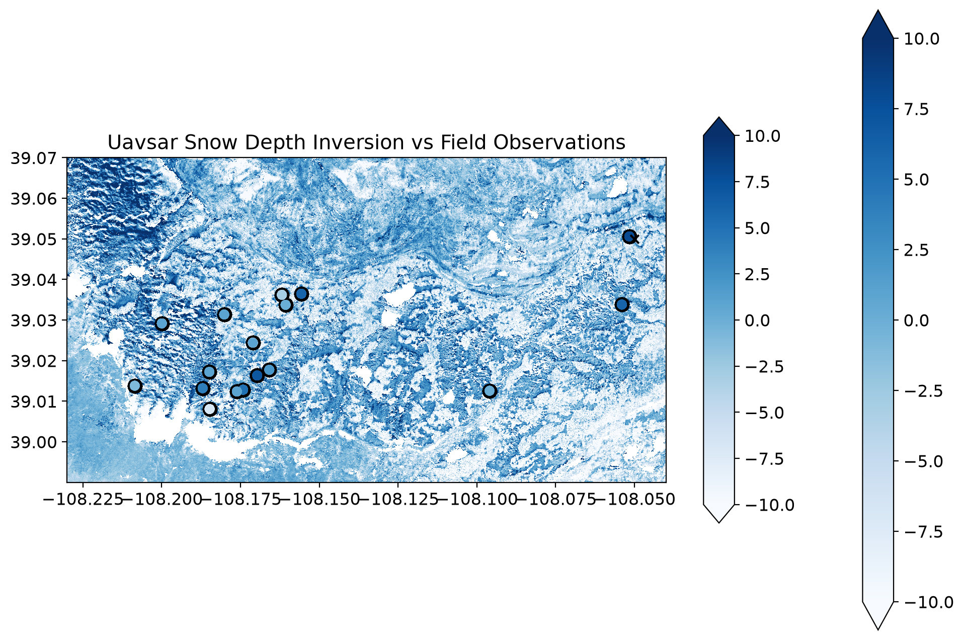

Numerical Comparison¶

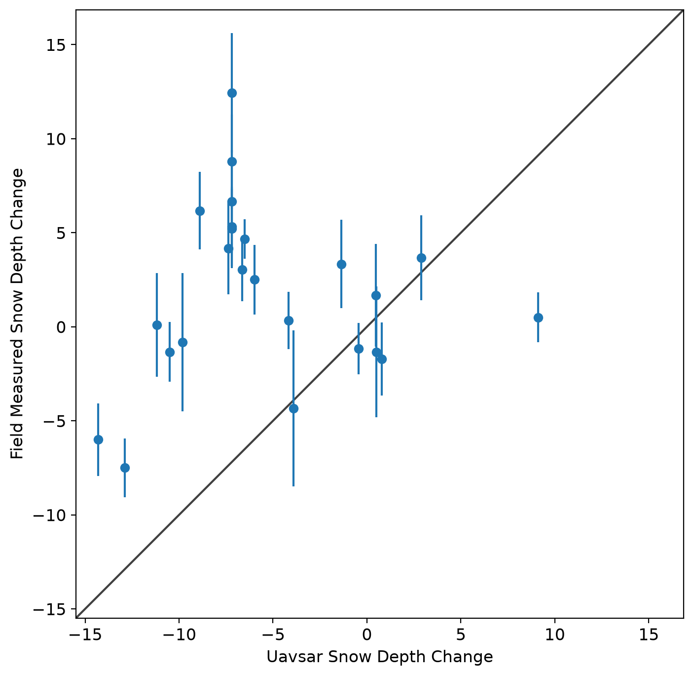
We can now extract the snow depth change at each measured point and compare them to the pit values of snow depth change.

# Sample UAVSAR snow depth change at field measurement points (in memory, no file I/O)
coord_list = [(x, y) for x, y in zip(df_both['geometry'].x, df_both['geometry'].y)]

# Use rioxarray to sample values directly from the in-memory array
from rasterio.transform import rowcol
df_both['uavsar_sd'] = [
    sd_change.sel(x=x, y=y, method='nearest').values.item() 
    for x, y in coord_list
]

f, ax = plt.subplots(figsize = (12,8))
df_both['geometry-str'] = df_both['geometry'].astype(str)
df_dis = df_both.dissolve('geometry-str', aggfunc={'sd_diff': 'mean', 'uavsar_sd': 'mean'})
field_sd_std = df_both.dissolve('geometry-str', aggfunc={'sd_diff': 'std'})['sd_diff'].values
ax.errorbar(x = df_dis.uavsar_sd, y = df_dis.sd_diff, yerr = field_sd_std, fmt="o")

lims = [
    np.min([ax.get_xlim(), ax.get_ylim()]),  # min of both axes
    np.max([ax.get_xlim(), ax.get_ylim()]),  # max of both axes
]
def rmse(predictions, targets):
    return np.sqrt(((predictions - targets) ** 2).mean())
rmse_sd = rmse(df_both['sd_diff'], df_both['uavsar_sd'])
print(f'RMSE between uavsar and field observations is {rmse_sd} cm')

# now plot both limits against each other
ax.plot(lims, lims, 'k-', alpha=0.75, zorder=0)
ax.set_aspect('equal')
ax.set_xlim(lims)
ax.set_ylim(lims)
ax.set_xlabel('Uavsar Snow Depth Change')
ax.set_ylabel('Field Measured Snow Depth Change')
plt.show()

RMSE between uavsar and field observations is 11.23737916931759 cm

Comparison to Lidar¶

# Create figures and subplots
fig, axes = plt.subplots(3, 1, figsize = (12,8))

# Load lidar data from S3
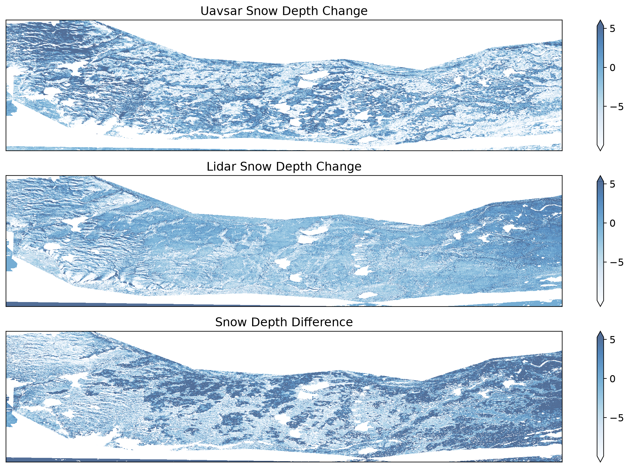
lidar = rxa.open_rasterio(S3_BASE_URL + 'sd_lidar.tif')

diff = lidar.copy()
diff = diff - sd_change

vmin, vmax = sd_change.quantile([0.1,0.9])
sd_change_masked = sd_change.copy()
sd_change_masked.data[np.isnan(lidar).data] = np.nan
sd_change_masked.plot(ax = axes[0], vmin = vmin, vmax = vmax, cmap = 'Blues', zorder = 1, alpha = 0.7)
lidar.plot(ax = axes[1], vmin = vmin, vmax = vmax, cmap = 'Blues', zorder = 1, alpha = 0.7)
diff.plot(ax = axes[2], vmin = vmin, vmax = vmax, cmap = 'Blues', zorder = 1, alpha = 0.7)

for ax in axes:
    ax.xaxis.set_visible(False)
    ax.yaxis.set_visible(False)

axes[0].set_title('Uavsar Snow Depth Change')
axes[1].set_title('Lidar Snow Depth Change')
axes[2].set_title('Snow Depth Difference')
plt.tight_layout()
plt.show()

/home/runner/micromamba/envs/snow-observations-cookbook/lib/python3.14/site-packages/matplotlib/colors.py:824: RuntimeWarning: overflow encountered in multiply
  xa *= self.N

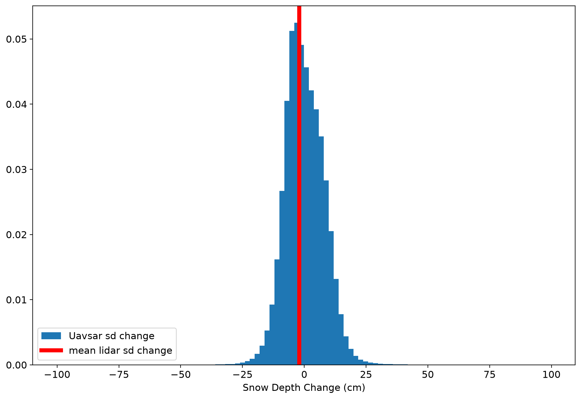
plt.figure(figsize = (12,8))
diffs = diff.values.ravel()
diffs = diffs[diffs < 100]
diffs = diffs[diffs > -100]
plt.hist(diffs, bins = 100, density = True, label = 'Uavsar sd change')
# plt.axvline(sd_change_masked.mean().values, label = 'Uavsar Mean Snow Depth Change', color = 'green')
lidar_vals = lidar.astype(np.float64).values[~lidar.isnull().values]
lidar_vals = lidar_vals[lidar_vals < 100]
lidar_vals = lidar_vals[lidar_vals > -100]
mean_lidar = np.nanmean(lidar_vals)
plt.axvline(mean_lidar, color = 'red', linewidth = 5, label = 'mean lidar sd change')
# plt.axvline(mean_lidar, label = 'Lidar Mean Snow Depth Change', color = 'red')
rmse = np.sqrt(((diffs) ** 2).mean())
print(f'Lidar mean depth change: {sd_change_masked.mean().values} cm, uavsar mean depth change: {mean_lidar} cm')
print(f'Mean difference: {np.nanmean(diffs)} cm, rmse = {rmse} cm')
plt.legend(loc = 'lower left')
plt.xlabel('Snow Depth Change (cm)')
plt.show()

Lidar mean depth change: -2.0986128849027437 cm, uavsar mean depth change: -2.0491660011047843 cm
Mean difference: 0.12355816024979177 cm, rmse = 8.070378174806594 cm