Basics of virtual Zarr stores

Overview

This notebook is intended as an introduction to creating and using virtual Zarr stores. In this tutorial we will:

Scan a single NetCDF4/HDF5 file to create a virtual dataset
Learn how to use the output using Xarray and Zarr.

While this notebook only examines using VirtualiZarr and Kerchunk on a single NetCDF file, these libraries can be used to create virtual Zarr datasets from collections of many input files. In the following notebook, we will demonstrate this.

Prerequisites

Concepts	Importance	Notes
Introduction to Xarray	Helpful	Basic features

Time to learn: 60 minutes

Imports

Here we will import a few Python libraries to help with our data processing.

virtualizarr will be used to generate the virtual Zarr store
Xarray for examining the output dataset

import xarray as xr
from virtualizarr import open_virtual_dataset

Define storage_options arguments

In the dictionary definition in the next cell, we are defining the options that will be passed to fsspec.open. Any additional kwargs passed in this dictionary through fsspec.open will pass as kwargs to the file system, in our case s3. The API docs for the s3fs filesystem spec can be found here.

In this example we are passing a few kwargs. In short they are:

anon=True: This is a s3fs kwarg that specifies you are not passing any connection credentials and are connecting to a public bucket.
default_fill_cache=False: s3fs kwarg that avoids caching in between chunks of files. This may lower memory usage when reading large files.
default_cache_type="none": fsspec kwarg that specifies the caching strategy used by fsspec. In this case, we turn off caching entirely to lower memory usage when only using the information from the file once…

storage_options = dict(anon=True, default_fill_cache=False, default_cache_type="none")

Virtualize a single NetCDF file

Below we will virtualize a NetCDF file stored on the AWS cloud. This dataset is a single time slice of a climate downscaled product for Alaska.

The steps in the cell below are as follows:

Create a virtual dataset using open_virtual_dataset
Write the virtual store as a Kerchunk reference JSON using the to_kerchunk method.

# Input URL to dataset. Note this is a netcdf file stored on s3 (cloud dataset).
url = "s3://wrf-se-ak-ar5/ccsm/rcp85/daily/2060/WRFDS_2060-01-01.nc"


# Create a virtual dataset using VirtualiZarr.
# We specify `indexes={}` to avoid creating in-memory pandas indexes for each 1D coordinate, since concatenating with pandas indexes is not yet supported in VirtualiZarr
virtual_ds = open_virtual_dataset(
    url, indexes={}, reader_options={"storage_options": storage_options}
)
# Write the virtual dataset to disk as a Kerchunk JSON. We could alternative write to a Kerchunk JSON or Icechunk Store.
virtual_ds.virtualize.to_kerchunk("single_file_kerchunk.json", format="json")

Opening virtual datasets

In the section below we will use the previously created Kerchunk reference JSON to open the NetCDF file as if it were a Zarr dataset.

# We once again need to provide information for fsspec to access the remote file
storage_options = dict(
    remote_protocol="s3", remote_options=dict(anon=True), skip_instance_cache=True
)
# We will use the "kerchunk" engine in `xr.open_dataset` and pass the `storage_options` to the `kerchunk` engine through `backend_kwargs`
ds = xr.open_dataset(
    "single_file_kerchunk.json",
    engine="kerchunk",
    backend_kwargs={"storage_options": storage_options},
)
ds

Plot dataset

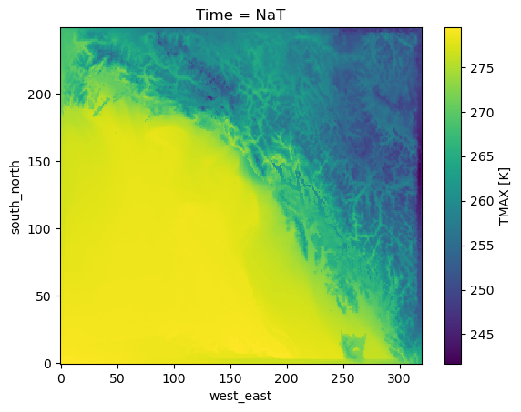
ds.TMAX.plot()

<matplotlib.collections.QuadMesh at 0x7f6ffb532e60>

../../_images/add2a98fb738e3a1d3d778c88308e5d8a8e6289cbe287435bbc79a7b749c6dbf.png

Note that the original .nc file size here is 16.8MB, and the created JSON is 26.5kB. These files also tend to compress very well. As you can see, it the JSON can be written anywhere, and gives us access to the underlying data, reading only the chunks we need from remote without downloading the whole file.