The Discrete Fourier Transform - Spectral Analysis for Geophysical Data Cookbook

Overview¶

The Discrete Fourier Transform (DFT) takes a signal made of evenly-spaced samples and breaks it into a sum of sines and cosines. For each wave in that sum, the DFT tells us three things:

the amplitude: how strong the wave is,
the frequency (or period): how fast it repeats,
the phase: where in the cycle it starts.

This short notebook covers the basics you need before moving on to power spectra and filtering:

The DFT formula and what its numbers mean.
Frequency, period, and the Nyquist limit.
A simple example: getting back the amplitudes, frequencies, and phases of a known signal.

Prerequisites¶

Concepts	Importance	Notes
Harmonic Analysis of the Seasonal Cycle	Helpful	Introduces sin/cos representation of the seasonal cycle
Remove the seasonal cycle using harmonic regression	Helpful	Removes seasonal cycle using harmonic regression

Time to learn: ~15 minutes

Imports¶

import numpy as np
import matplotlib.pyplot as plt
import seaborn as sns

sns.set_theme(style="whitegrid", context="notebook", font_scale=1.2)

From continuous to discrete¶

Say we have a real signal made of $N$ samples $x_0, x_1, \dots, x_{N-1}$ , taken every $\Delta t$ seconds. The Discrete Fourier Transform is the formula

\hat{x}_k \;=\; \sum_{n=0}^{N-1} x_n \, e^{-i\, 2\pi k n / N}, \qquad k = 0, 1, \dots, N-1.

(1)

Each $\hat{x}_k$ is a complex number that describes one wave inside the signal:

Amplitude (how big the wave is): $A_k = \dfrac{2}{N}\,|\hat{x}_k|$ (for $0 < k < N/2$ ).
Phase (where the wave starts): $\varphi_k = \arg(\hat{x}_k)$ .

We can also go back from the coefficients to the original samples, no information is lost:

x_n \;=\; \frac{1}{N}\sum_{k=0}^{N-1} \hat{x}_k \, e^{\,i\, 2\pi k n / N}.

(2)

Frequency, period, and Nyquist¶

The index $k$ matches a real-world frequency:

f_k \;=\; \frac{k}{N\,\Delta t}, \qquad \text{period} \;=\; \frac{1}{f_k} = \frac{N\,\Delta t}{k}.

(3)

The fastest wave we can detect with our sampling is the Nyquist frequency:

f_{\text{Nyq}} \;=\; \frac{1}{2\,\Delta t}.

(4)

Any wave that wiggles faster than this will look like a slower wave in our data, this is called aliasing. Because the spectrum of a real signal is mirrored around the center, only the first $N/2 + 1$ coefficients carry new information. That is what numpy.fft.rfft gives back.

A worked example: a sum of two sines¶

Let’s build a fake signal with two waves we already know about, plus a constant value:

x(t) \;=\; 5 \;+\; 3\,\cos(2\pi\, f_1 t) \;+\; 2\,\sin(2\pi\, f_2 t),

(5)

with $f_1 = 2$ Hz and $f_2 = 5$ Hz. If the DFT works, it should find exactly these two frequencies with the right amplitudes.

fs = 100.0
T = 2.0
N = int(fs * T)
dt = 1.0 / fs
t = np.arange(N) * dt

f1, A1 = 2.0, 3.0
f2, A2 = 5.0, 2.0
offset = 5.0

x = offset + A1 * np.cos(2 * np.pi * f1 * t) + A2 * np.sin(2 * np.pi * f2 * t)

fig, ax = plt.subplots(figsize=(8, 3))
ax.plot(t, x, color="C0")
ax.set_xlabel("Time (s)")
ax.set_ylabel("x(t)")
ax.set_title("Synthetic signal")
plt.show()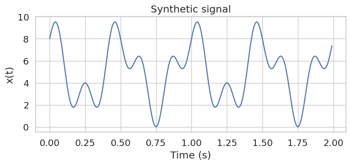

Compute the DFT¶

Since our signal is real-valued, we use numpy.fft.rfft. It only returns the positive-frequency coefficients (the negative ones would be a mirror copy). numpy.fft.rfftfreq gives us the matching frequencies in Hz.

X = np.fft.rfft(x)
freqs = np.fft.rfftfreq(N, d=dt)

amplitude = (2.0 / N) * np.abs(X)
amplitude[0] = np.abs(X[0]) / N

phase = np.angle(X)

fig, ax = plt.subplots(figsize=(8, 3))
ax.stem(freqs, amplitude, basefmt=" ")
ax.set_xlim(1, 10)
ax.set_xticks(np.arange(1, 11, 1))
ax.set_xlabel("Frequency (Hz)")
ax.set_ylabel("Amplitude")
ax.set_title("Amplitude spectrum")
plt.show()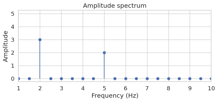

The two peaks fall right at 2 Hz and 5 Hz, with amplitudes 3 and 2, just as we set them. The value at 0 Hz is the mean of the signal (5). To get the period of each peak, we just take $1/f$ :

peak_idx = np.argsort(amplitude[1:])[-2:] + 1

for k in sorted(peak_idx):
    print(
        f"k={k:3d}  f={freqs[k]:5.2f} Hz  "
        f"period={1/freqs[k]:5.2f} s  "
        f"amplitude={amplitude[k]:.2f}  "
        f"phase={np.degrees(phase[k]):+6.1f}°"
    )

k=  4  f= 2.00 Hz  period= 0.50 s  amplitude=3.00  phase=  -0.0°
k= 10  f= 5.00 Hz  period= 0.20 s  amplitude=2.00  phase= -90.0°

Reconstructing the signal¶

The DFT can be undone, so feeding the coefficients into np.fft.irfft gives us back the original samples (with only tiny rounding errors).

x_reconstructed = np.fft.irfft(X, n=N)
max_error = np.max(np.abs(x - x_reconstructed))
print(f"Maximum reconstruction error: {max_error:.2e}")

Maximum reconstruction error: 4.00e-15

Summary¶

The DFT splits a sampled signal into a set of complex numbers. Each one describes one wave by giving its amplitude, frequency (and so its period), and phase. The transform is exact and reversible, and the fastest wave we can see depends on the sampling rate through the Nyquist limit.

What’s next?¶

Now that we know the DFT, we can square the coefficients to get a power spectrum, find the dominant time scales in a climate time series, and build filters that keep or remove certain frequency bands. That is what we do in Fourier Power Spectrum and Spectral Filtering.