Remove the seasonal cycle using harmonic regression - Spectral Analysis for Geophysical Data Cookbook

Overview¶

Many geophysical time series carry a strong seasonal cycle. Before studying variability on other time scales (intraseasonal, interannual, or trends) we often want anomalies: departures from that repeating seasonal pattern.

One practical way to remove the seasonal cycle is harmonic regression. The idea is to represent the annual signal as a sum of sine and cosine waves at integer multiples of one cycle per year, then estimate the contribution of each harmonic by projecting the data onto that basis.

In this notebook we:

Load daily outgoing longwave radiation (OLR) and extract a single time series.
Build a design matrix whose columns are a constant term plus sin/cos pairs for the first few annual harmonics.
Project the time series onto those columns with least squares to obtain the fitted seasonal cycle.
Subtract the fitted cycle to obtain anomalies.

The same workflow extends directly to gridded data: each grid point is regressed against the same harmonic basis.

Prerequisites¶

Concepts	Importance	Notes
Harmonic Analysis of the Seasonal Cycle	Helpful	Introduces sin/cos representation of the seasonal cycle
Linear least squares	Necessary	Coefficients are estimated by projection onto harmonic basis functions

Time to learn: ~20 minutes

Imports¶

All packages used in the rest of the notebook are imported up front. s3fs is configured to read anonymously from the public Pythia bucket on the Jetstream2 S3 endpoint.

import numpy as np
import pandas as pd
import matplotlib.pyplot as plt
import seaborn as sns

import s3fs
import xarray as xr

sns.set_theme(style="whitegrid", context="notebook", font_scale=1.2)

URL = "https://js2.jetstream-cloud.org:8001/"
fs = s3fs.S3FileSystem(anon=True, client_kwargs=dict(endpoint_url=URL))

Load NOAA OLR¶

We use daily Outgoing Longwave Radiation (OLR) from NOAA Lee & others, 2014, stored as a Zarr dataset on the Pythia Jetstream2 bucket. OLR is a common proxy for tropical convection and shows a clear annual cycle at many locations.

olr_noaa_store = s3fs.S3Map(
    root="pythia/olr_noaa.zarr",
    s3=fs,
    check=False,
)

# Open with xarray
olr_noaa = xr.open_zarr(olr_noaa_store)
olr_noaa = olr_noaa.rename_vars({"__xarray_dataarray_variable__": "olr"})

olr_noaa = olr_noaa.chunk({"time": -1})
olr_noaa = olr_noaa.interpolate_na(dim="time", method="linear")

Select a time series¶

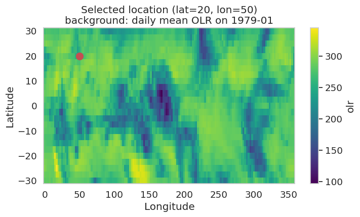
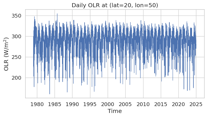
We pick one grid point in the tropics and inspect its daily OLR record. The map below marks the selected location; the next plot shows the full time series at that point.

lat_select = 20
lon_select = 50

olr_band_series = olr_noaa["olr"].sel(
    lat=lat_select, lon=lon_select, method="nearest"
)

time_value = pd.to_datetime(olr_band_series.time[0].values)

fig, ax = plt.subplots(figsize=(8, 4))
olr_noaa["olr"][0].plot(ax=ax)
ax.plot(lon_select, lat_select, "ro", markersize=10)
ax.set_title(
    f"Selected location (lat={lat_select}, lon={lon_select})\n"
    f"background: daily mean OLR on {time_value:%Y-%m}"
)
ax.set_xlabel("Longitude")
ax.set_ylabel("Latitude")
plt.show()

fig, ax = plt.subplots(figsize=(8, 4))
olr_band_series.plot(ax=ax, color="C0", linewidth=0.8)
ax.set_title(f"Daily OLR at (lat={lat_select}, lon={lon_select})")
ax.set_xlabel("Time")
ax.set_ylabel("OLR (W/m$^2$)")
plt.show()

series = olr_band_series.values
n_time = len(series)
print(f"Time series length: {n_time} days")

Time series length: 16802 days

Build the harmonic design matrix¶

Suppose the observed series is $y(t)$ and we want to isolate variability that repeats every $T$ time units. For daily data, we typically use $T = 365.25$ days to represent the annual cycle. The value 365.25 accounts for leap years by including the average extra quarter day per year over the Gregorian calendar. For monthly-mean data, the annual cycle has a period of $T = 12$ months, since the time coordinate advances in monthly increments rather than days.

A truncated harmonic expansion with $K$ pairs of sine and cosine terms is

y(t) \approx a_0 + \sum_{k=1}^{K} \left[ a_k \sin\!\left(\frac{2\pi k t}{T}\right) + b_k \cos\!\left(\frac{2\pi k t}{T}\right) \right].

(1)

Each basis function is one column of a design matrix $\mathbf{X} \in \mathbb{R}^{n \times (2K+1)}$ :

\mathbf{X} = \begin{bmatrix} \mathbf{1} & \sin\!\left(\frac{2\pi t}{T}\right) & \cos\!\left(\frac{2\pi t}{T}\right) & \cdots & \sin\!\left(\frac{2\pi K t}{T}\right) & \cos\!\left(\frac{2\pi K t}{T}\right) \end{bmatrix}.

(2)

The first column is a constant (mean level). The $k$ -th harmonic completes $k$ full cycles over one year; higher harmonics let the fitted seasonal cycle depart from a simple cosine shape.

Stacking the data as a vector $\mathbf{y}$ , the least-squares coefficients are the projection of $\mathbf{y}$ onto the column space of $\mathbf{X}$ :

\mathbf{c} = \underset{\mathbf{c}}{\arg\min} \, \lVert \mathbf{y} - \mathbf{X}\mathbf{c} \rVert_2^2.

(3)

In code this is a single call to np.linalg.lstsq. The fitted seasonal cycle is $\hat{\mathbf{y}}_{\text{seasonal}} = \mathbf{X}\mathbf{c}$ , and the anomalies are the residual $\mathbf{y} - \hat{\mathbf{y}}_{\text{seasonal}}$ .

n_harmonics = 4
year_period = 365.25  # days

t = np.arange(n_time)
X = np.ones((n_time, 2 * n_harmonics + 1))
for i in range(1, n_harmonics + 1):
    X[:, 2 * i - 1] = np.sin(i * 2 * np.pi * t / year_period)
    X[:, 2 * i] = np.cos(i * 2 * np.pi * t / year_period)

print(f"Design matrix shape: {X.shape}")

Design matrix shape: (16802, 9)

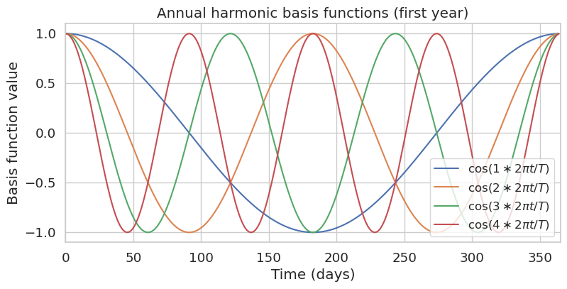
The plot below shows the first-year segment of the cosine basis functions. Together with their sine partners and the constant column, they span the seasonal subspace we project onto.

fig, ax = plt.subplots(figsize=(9, 4))
for i in range(1, n_harmonics + 1):
    ax.plot(t[: int(year_period)], X[: int(year_period), 2 * i],
            label=fr"$\cos({i} \ast  2\pi t/T)$")
ax.set_xlim(0, year_period)
ax.legend(loc="lower right", fontsize=12)
ax.set_xlabel("Time (days)")
ax.set_ylabel("Basis function value")
ax.set_title("Annual harmonic basis functions (first year)")
plt.show()

Project the data and compute anomalies¶

We now solve for the coefficient vector $\mathbf{c}$ and form the fitted seasonal cycle and anomalies. Increasing n_harmonics allows a more flexible seasonal shape; in practice $K = 3$ –4 is often enough for daily climate data.

coeffs = np.linalg.lstsq(X, series, rcond=None)[0]
annual_cycle = X @ coeffs
anomalies = series - annual_cycle

print(f"Coefficient vector length: {len(coeffs)}")

Coefficient vector length: 9

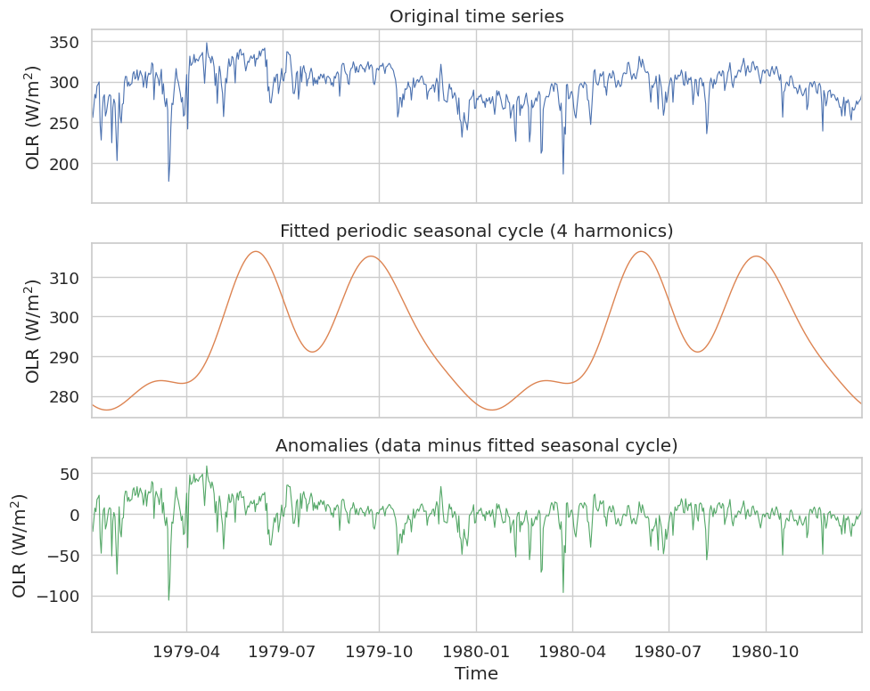
The figure below compares the original series, the harmonic fit (projection onto $\mathbf{X}$ ), and the resulting anomalies.

fig, axes = plt.subplots(3, 1, figsize=(10, 8), sharex=True)

axes[0].plot(olr_band_series.time, series, color="C0", linewidth=0.8)
axes[0].set_ylabel("OLR (W/m$^2$)")
axes[0].set_title("Original time series")
axes[0].set_xlim(olr_band_series.time.isel(time=0),
                 olr_band_series.time.isel(time=int(year_period*2)))

axes[1].plot(olr_band_series.time, annual_cycle, color="C1", linewidth=1.0)
axes[1].set_ylabel("OLR (W/m$^2$)")
axes[1].set_title(f"Fitted periodic seasonal cycle ({n_harmonics} harmonics)")
axes[1].set_xlim(olr_band_series.time.isel(time=0),
                 olr_band_series.time.isel(time=int(year_period*2)))

axes[2].plot(olr_band_series.time, anomalies, color="C2", linewidth=0.8)
axes[2].set_ylabel("OLR (W/m$^2$)")
axes[2].set_xlabel("Time")
axes[2].set_title("Anomalies (data minus fitted seasonal cycle)")
axes[2].set_xlim(olr_band_series.time.isel(time=0),
                 olr_band_series.time.isel(time=int(year_period*2)))

fig.tight_layout()
plt.show()

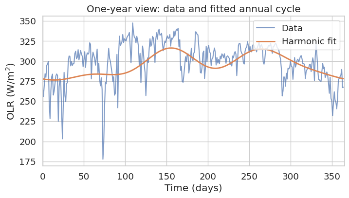
Zooming into one year makes the harmonic fit easier to compare with the raw signal.

one_year = slice(0, int(year_period))
days = t[one_year]

fig, ax = plt.subplots(figsize=(8, 4))
ax.plot(days, series[one_year], color="C0", alpha=0.7, label="Data")
ax.plot(days, annual_cycle[one_year], color="C1", linewidth=2, label="Harmonic fit")
ax.set_xlim(0, year_period)
ax.set_xlabel("Time (days)")
ax.set_ylabel("OLR (W/m$^2$)")
ax.set_title("One-year view: data and fitted annual cycle")
ax.legend(loc="upper right")
plt.show()

Apply to gridded data¶

The single-grid-point workflow generalizes directly to a full 3D field $\mathbf{Y} \in \mathbb{R}^{n_t \times n_{\text{lat}} \times n_{\text{lon}}}$ . Because the design matrix $\mathbf{X}$ does not depend on space, the same basis is shared by every grid point, the only thing that changes from one grid point to the next is the coefficient vector $\mathbf{c}$ .

field_3d = olr_noaa['olr'].values  # shape: (time, lat, lon)
n_t, n_lat, n_lon = field_3d.shape

field_2d = field_3d.reshape(n_t, n_lat * n_lon)

coeffs_grid = np.linalg.lstsq(X, field_2d, rcond=None)[0]
seasonal_grid = (X @ coeffs_grid).reshape(n_t, n_lat, n_lon)
anomalies_grid = field_3d - seasonal_grid

olr_anom = xr.DataArray(
    anomalies_grid,
    coords=olr_noaa['olr'].coords,
    dims=olr_noaa['olr'].dims,
    name="olr_anom",
    attrs={'long_name': 'OLR anomalies', 'units': 'W/m^2'},
)

olr_anom[0].plot()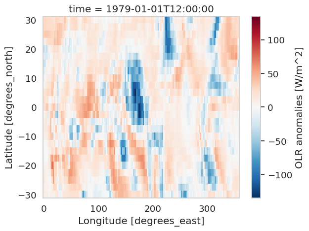

Summary¶

Harmonic regression removes the seasonal cycle by projecting a time series onto a matrix of annual sin/cos basis functions plus a constant term. The fitted seasonal cycle lives in the column space of that design matrix; subtracting it leaves anomalies that are orthogonal (in a least-squares sense) to the seasonal subspace.

Key steps:

Choose the period $T$ and number of harmonics $K$ .
Build $\mathbf{X}$ with one column per basis function.
Solve $\mathbf{c} = \arg\min \lVert \mathbf{y} - \mathbf{X}\mathbf{c} \rVert_2^2$ .
Compute anomalies as $\mathbf{y} - \mathbf{X}\mathbf{c}$ .

The same design matrix can be applied to every grid point in a field.

What’s next?¶

With the seasonal cycle removed, the anomalies are ready for analysis on other time scales (intraseasonal, interannual, and longer).

The next notebook, The Discrete Fourier Transform, introduces the DFT as the natural tool for that step: it generalizes the harmonic basis used here to all frequencies resolvable by the sampling, and returns the amplitude, period, and phase of each component. Those coefficients are the building blocks for the power spectrum and spectral filtering that follow in later notebooks.

References¶

Lee, H.-T., & others. (2014). NOAA climate data record (CDR) of daily outgoing longwave radiation (OLR), version 1.2. (No Title).