Limitation of the Fourier transform and Fourier series: The Gibbs Phenomenon - Spectral Analysis for Geophysical Data Cookbook

Overview¶

When a Fourier series is used to approximate a function with a jump discontinuity, the partial sums do not converge uniformly near the discontinuity. Instead, they overshoot the true value of the function on either side of the jump by a fixed proportion no matter how many terms are added. This persistent overshoot, which becomes narrower but never smaller in amplitude as more modes are included, is known as the Gibbs phenomenon.

The code in this notebook is adapted from Brunton & Kutz (2022)

Prerequisites¶

Concepts	Importance	Notes
The Discrete Fourier Transform	Needed	Introduces sin/cos representation of the seasonal cycle
Fourier Power Spectrum and Spectral Filtering	Needed	Understanding the Fourier Transform Decomposition and Spectral Filtering

Time to learn: 10 minutes

Imports¶

import os
import numpy as np
import matplotlib.pyplot as plt
from matplotlib import animation, rc
from IPython.display import HTML
import seaborn as sns
sns.set_theme(style='whitegrid', context='notebook', font_scale=1.3,)

The square wave¶

dx = 0.01
L = 10
x = np.arange(0, L+dx, dx)
n = len(x)
nquart = int(np.floor(n/4)) # 1/4 of the total length

f = np.zeros_like(x)
f[nquart:3*nquart] = 1 # L/4 to 3L/4 is 1, 0 otherwise

plt.plot(x, f, color='k', linewidth=2)
plt.title('Square Wave')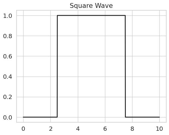

Fourier Series¶

Any reasonably well-behaved $L$ -periodic function $f(x)$ can be expanded as an infinite sum of sines and cosines:

f(x) = \frac{a_0}{2} + \sum_{k=1}^{\infty}\left( a_k\,\cos\!\left(\frac{2\pi k x}{L}\right) + b_k\,\sin\!\left(\frac{2\pi k x}{L}\right) \right)

(1)

The constant term $a_0/2$ is the average value of $f$ over one period, and each pair $(a_k, b_k)$ gives the contribution of the $k$ -th harmonic, a wave whose period is $L/k$ .

The coefficients are obtained by projecting $f$ onto each basis function (using the orthogonality of sines and cosines on $[0, L]$ ):

a_k = \frac{2}{L}\int_{0}^{L} f(x)\,\cos\!\left(\frac{2\pi k x}{L}\right) dx, \qquad b_k = \frac{2}{L}\int_{0}^{L} f(x)\,\sin\!\left(\frac{2\pi k x}{L}\right) dx.

(2)

In the code below these integrals are approximated by Riemann sums over the discrete grid (np.sum(...) * dx). A truncated series with $K$ modes,

f_K(x) = \frac{a_0}{2} + \sum_{k=1}^{K}\left( a_k\,\cos\!\left(\frac{2\pi k x}{L}\right) + b_k\,\sin\!\left(\frac{2\pi k x}{L}\right) \right)

(3)

Approximate the square wave¶

# A0 is the projection of f onto the constant basis function (cos(0) = 1)
k = 0
A0 = np.sum(f * np.cos(np.pi*(k)*x/L)) * dx * 2 / L
fFS = A0/2 * np.ones_like(f)

fig, ax = plt.subplots()
ax.plot(x, f, color='k', linewidth=2)
fFS_plot, = ax.plot([], [], color='r', linewidth=2)

all_fFS = np.zeros((len(fFS), 101))
all_fFS[:, 0] = fFS

# A[k] and B[k] are the cosine and sine Fourier coefficients for mode k+1.
for k in range(1, 101):
    Ak = np.sum(f * np.cos(2*np.pi*k*x/L)) * dx * 2 / L
    Bk = np.sum(f * np.sin(2*np.pi*k*x/L)) * dx * 2 / L
    fFS = fFS + Ak*np.cos(2*k*np.pi*x/L) + Bk*np.sin(2*k*np.pi*x/L)
    all_fFS[:, k] = fFS


def init():
    ax.set_xlim(x[0], x[-1])
    ax.set_ylim(-0.2, 1.2)
    return fFS


def animate(iter):
    fFS_plot.set_data(x, all_fFS[:, iter])
    ax.set_title(f'k={iter:03d}')
    return fFS_plot


anim = animation.FuncAnimation(fig, animate, init_func=init,
                               frames=101, interval=50, blit=False,
                               repeat=False)

plt.close(fig)
HTML(anim.to_jshtml())

In the example above, the square wave (discontinuos Hat Function) is reconstructed from its Fourier series. As the number of modes $k$ increases, the approximation becomes more accurate in the smooth regions, but characteristic “ears” remain at the edges of the discontinuity. This illustrates a fundamental limitation of Fourier representations for piecewise-smooth signals.

Summary¶

A truncated Fourier series can represent any smooth periodic function arbitrarily well, but it cannot fully resolve a jump discontinuity. Near each jump the partial sums systematically overshoot the true value by about 9% of the jump height, and this overshoot does not shrink as more modes are added, it only becomes narrower. This is the Gibbs phenomenon, and it is a fundamental property of any series expansion in a smooth (sine/cosine) basis. In practice, it warns us that Fourier-based reconstructions, power spectra, and spectral filters should be interpreted with care whenever the underlying signal contains sharp transitions, fronts, regime shifts, or finite-record edges.

What’s next?¶

Having completed the Fourier-based portion of the cookbook, we now switch to a different decomposition that is better suited to spatially-organized geophysical fields: Empirical Orthogonal Functions (EOFs). The next notebook, EOF Analysis in 2D, introduces EOFs on a simple synthetic dataset and builds the intuition we will reuse for the 3D and multivariate examples that follow.

References¶

Brunton, S. L., & Kutz, J. N. (2022). Data-Driven Science and Engineering : Machine Learning, Dynamical Systems, and Control.