Fourier Power Spectrum and Spectral Filtering - Spectral Analysis for Geophysical Data Cookbook

Overview¶

The Fourier transform decomposes a time series into sine and cosine waves at different frequencies. The power spectrum shows how much variance each frequency explains, useful for spotting the annual cycle, intraseasonal variability, and other climate signals.

In this notebook we:

Load daily OLR at a single grid point.
Compute and interpret the power spectrum of that pixel time series.
Apply low-pass, high-pass, and band-pass filters in frequency space.

Prerequisites¶

Concepts	Importance	Notes
Remove the seasonal cycle using harmonic regression	Helpful	Same OLR dataset and pixel-selection workflow
Discrete Fourier transform	Necessary	Amplitude, frequency, and period

Time to learn: ~25 minutes

Imports¶

All packages are imported up front. s3fs reads anonymously from the public Pythia bucket on the Jetstream2 S3 endpoint.

import numpy as np
import pandas as pd
import matplotlib.pyplot as plt
import seaborn as sns

import s3fs
import xarray as xr

sns.set_theme(style="whitegrid", context="notebook", font_scale=1.2)

URL = "https://js2.jetstream-cloud.org:8001/"
fs = s3fs.S3FileSystem(anon=True, client_kwargs=dict(endpoint_url=URL))

Load NOAA OLR¶

We use daily Outgoing Longwave Radiation (OLR) from NOAA Lee & others, 2014, stored as a Zarr dataset on the Pythia Jetstream2 bucket, the same source as in harmonic anomalies.

olr_noaa_store = s3fs.S3Map(
    root="pythia/olr_noaa.zarr",
    s3=fs,
    check=False,
)

olr_noaa = xr.open_zarr(olr_noaa_store)
olr_noaa = olr_noaa.rename_vars({"__xarray_dataarray_variable__": "olr"})
olr_noaa = olr_noaa.chunk({"time": -1})
olr_noaa = olr_noaa.interpolate_na(dim="time", method="linear")

Select a single-pixel time series¶

Spectral analysis starts with one location. We pick a tropical grid point and remove the time mean so the FFT focuses on variability rather than the absolute OLR level.

lat_select = 20
lon_select = 50

olr_series = olr_noaa["olr"].sel(
    lat=lat_select, lon=lon_select, method="nearest"
)
series = olr_series.values
series_centered = series - series.mean()
n_time = len(series)

fig, ax = plt.subplots(figsize=(8, 3))
olr_series.plot(ax=ax, color="C0", linewidth=0.8)
ax.set_title(f"Daily OLR at (lat={lat_select}, lon={lon_select})")
ax.set_ylabel("OLR (W/m$^2$)")
plt.show()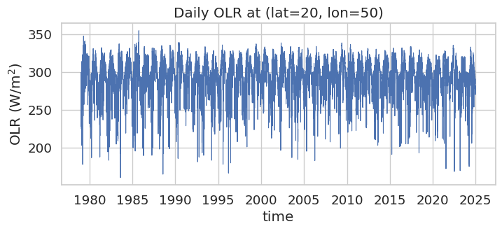

Compute the power spectrum¶

For a centered series $x(t)$ with sampling interval $\Delta t = 1$ day, the discrete Fourier transform gives complex coefficients $\hat{x}_k$ . The power at frequency $k$ is $|\hat{x}_k|^2$ . Summing power across all frequencies equals the series variance.

We convert frequency to period (days) with $\text{period} = 1 / |f|$ and express each bin as the fraction of total variance it explains. Peaks near 365 days mark the annual cycle and its harmonics.

def power_spectrum(series, dt=1.0):
    """Return positive-frequency periods (days) and explained variance (%)."""
    x = series - np.mean(series)
    n = len(x)
    freqs = np.fft.rfftfreq(n, d=dt)
    coeffs = np.fft.rfft(x)
    power = np.abs(coeffs) ** 2

    var = np.var(x)
    pct_var = 100.0 * power / power.sum() if power.sum() > 0 else power

    with np.errstate(divide="ignore"):
        periods = np.where(freqs > 0, 1.0 / freqs, np.inf)

    mask = freqs > 0
    return periods[mask], pct_var[mask], var


periods, pct_var, series_var = power_spectrum(series)
print(f"Series length: {n_time} days | variance: {series_var:.2f} (W/m$^2$)$^2$")

Series length: 16802 days | variance: 492.19 (W/m$^2$)$^2$

fig, ax = plt.subplots(figsize=(6, 4))
ax.plot(periods, pct_var, color="k", linewidth=1.6)
ax.set_xscale("log")
ax.set_xlim(10, n_time)
ax.set_xlabel("Period (days)")
ax.set_ylabel("Explained variance (%)")
ax.set_title("Power spectrum of a single OLR pixel")

for period, label, color in [
    (365.25, "1 year", "C3"),
    (365.25 / 2, "6 months", "C4"),
    (365.25 / 3, "4 months", "C5"),
    (365.25 / 4, "3 months", "C6"),
]:
    ax.axvline(period, color=color, linestyle="--", alpha=0.8, label=label, zorder=1)
ax.legend(loc="upper right")
plt.show()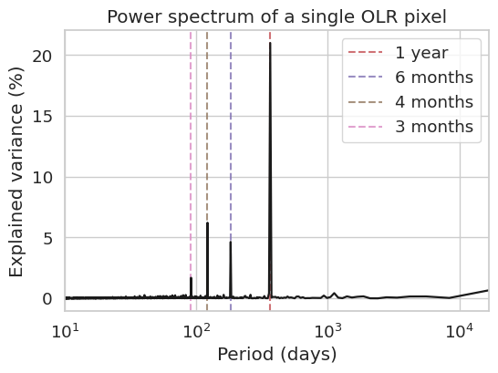

As we see, the largest peaks usually occur near the annual cycle and its harmonics. While this confirms that the seasonal cycle is the dominant source of variability, it offers little new insight, as this behavior is already well known.

To reveal variability beyond the seasonal cycle, we repeat the analysis using anomalies obtained after removing the annual cycle and its first four harmonics, following the procedure described in Remove the seasonal cycle using harmonic regression. This filtering suppresses the seasonal signal, allowing other modes of variability to emerge more clearly.

n_harmonics = 4
year_period = 365.25  # days

t = np.arange(n_time)
X = np.ones((n_time, 2 * n_harmonics + 1))
for i in range(1, n_harmonics + 1):
    X[:, 2 * i - 1] = np.sin(i * 2 * np.pi * t / year_period)
    X[:, 2 * i] = np.cos(i * 2 * np.pi * t / year_period)


coeffs = np.linalg.lstsq(X, series, rcond=None)[0]
annual_cycle = X @ coeffs
anomalies = series - annual_cycle

periods, pct_var_harmonics, series_var_harmonics = power_spectrum(anomalies)

fig, ax = plt.subplots(figsize=(6, 4))
ax.plot(periods, pct_var_harmonics, color="k", linewidth=1.6)
ax.set_xscale("log")
ax.set_xlim(2, n_time)
ax.set_xlabel("Period (days)")
ax.set_ylabel("Explained variance (%)")
ax.set_title("Power spectrum of a single OLR pixel")

for period, label, color in [
    (365.25, "1 year", "C3"),
    (365.25 / 2, "6 months", "C4"),
    (365.25 / 3, "4 months", "C5"),
    (365.25 / 4, "3 months", "C6"),
]:
    ax.axvline(period, color=color, linestyle="--", alpha=0.8, label=label, zorder=1)
ax.legend(loc="upper right")
plt.show()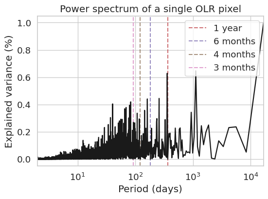

Now we see that the largest fraction of the explained variability is concentrated at low frequencies, corresponding to periods longer than 10⁴ days. A substantial amount of variance is also found in the interannual band (approximately 2–7 years), while another significant contribution arises from intraseasonal variability, with periods between about 20 and 90 days Zhang, 2013.

Spectral filtering¶

Spectral filtering isolates variability within a desired range of time scales by modifying the Fourier coefficients before transforming the signal back to the time domain. The procedure consists of three steps:

Compute the FFT of the mean-centered time series.
Retain only the Fourier coefficients corresponding to the desired period range.
Perform the inverse FFT and add the mean back to reconstruct the filtered signal.

Filter	Keeps periods	Typical use
Low-pass	longer than a cutoff	isolate slow variability (e.g., interannual to decadal)
High-pass	shorter than a cutoff	remove slow variations such as trends and the seasonal cycle
Band-pass	between two cutoffs	isolate a specific range of variability (e.g., MJO)

The helper function spectral_filter below implements this procedure using NumPy. After removing the time mean, it computes the real FFT (np.fft.rfft) and converts each frequency bin to its corresponding period, (T = 1/f). A boolean mask is then applied to determine which Fourier coefficients are retained.

The filtering options are:

Low-pass: specify period_min only, retaining periods $( T \geq T_{\min} )$ .
High-pass: specify period_max only, retaining periods $(T \leq T_{\max})$ .
Band-pass: specify both period_min and period_max, retaining periods $(T_{\min} \leq T \leq T_{\max})$ .

The zero-frequency (DC) component is always removed because the mean has already been subtracted. The filtered time series is then reconstructed with np.fft.irfft.

Below, we apply these filters to the harmonic anomalies, using a 100-day cutoff to separate low- and high-frequency variability and a 20–90 day band-pass filter to isolate intraseasonal fluctuations, including signals associated with the Madden–Julian Oscillation (MJO).

def spectral_filter(series, period_min=None, period_max=None, dt=1.0):
    """Band-pass in period space; omit period_min or period_max for high/low pass."""
    mean = np.mean(series)
    x = series - mean
    n = len(x)
    freqs = np.fft.rfftfreq(n, d=dt)
    coeffs = np.fft.rfft(x)

    with np.errstate(divide="ignore"):
        freq_periods = np.where(freqs > 0, 1.0 / freqs, np.inf)

    keep = np.ones_like(freqs, dtype=bool)
    if period_max is not None:
        keep &= freq_periods <= period_max
    if period_min is not None:
        keep &= freq_periods >= period_min
    keep[0] = False  # remove the DC (mean) component

    coeffs_filtered = np.where(keep, coeffs, 0.0)
    return np.fft.irfft(coeffs_filtered, n=n)


cutoff = 100  # days
bp_low, bp_high = 20, 90  # days

lowpass = spectral_filter(anomalies, period_min=cutoff)
highpass = spectral_filter(anomalies, period_max=cutoff)
bandpass = spectral_filter(anomalies, period_min=bp_low,
                           period_max=bp_high)

Compare the original series with each filtered version over two years. The low-pass trace follows the seasonal envelope; the high-pass trace removes it; the band-pass trace isolates intraseasonal swings.

two_years = slice(0, int(365.25 * 2))
time_slice = olr_series.time[two_years]

fig, axes = plt.subplots(4, 1, figsize=(10, 9), sharex=True)
panels = [
    (series[two_years], "Original", "C0"),
    (lowpass[two_years], f"Low-pass (periods > {cutoff} days)", "C1"),
    (highpass[two_years], f"High-pass (periods < {cutoff} days)", "C2"),
    (bandpass[two_years], f"Band-pass ({bp_low}–{bp_high} days)", "C3"),
]
for ax, (data, title, color) in zip(axes, panels):
    ax.plot(time_slice, data, color=color, linewidth=0.8)
    ax.set_ylabel("OLR (W/m$^2$)")
    ax.set_title(title)
axes[-1].set_xlabel("Time")
fig.tight_layout()
plt.show()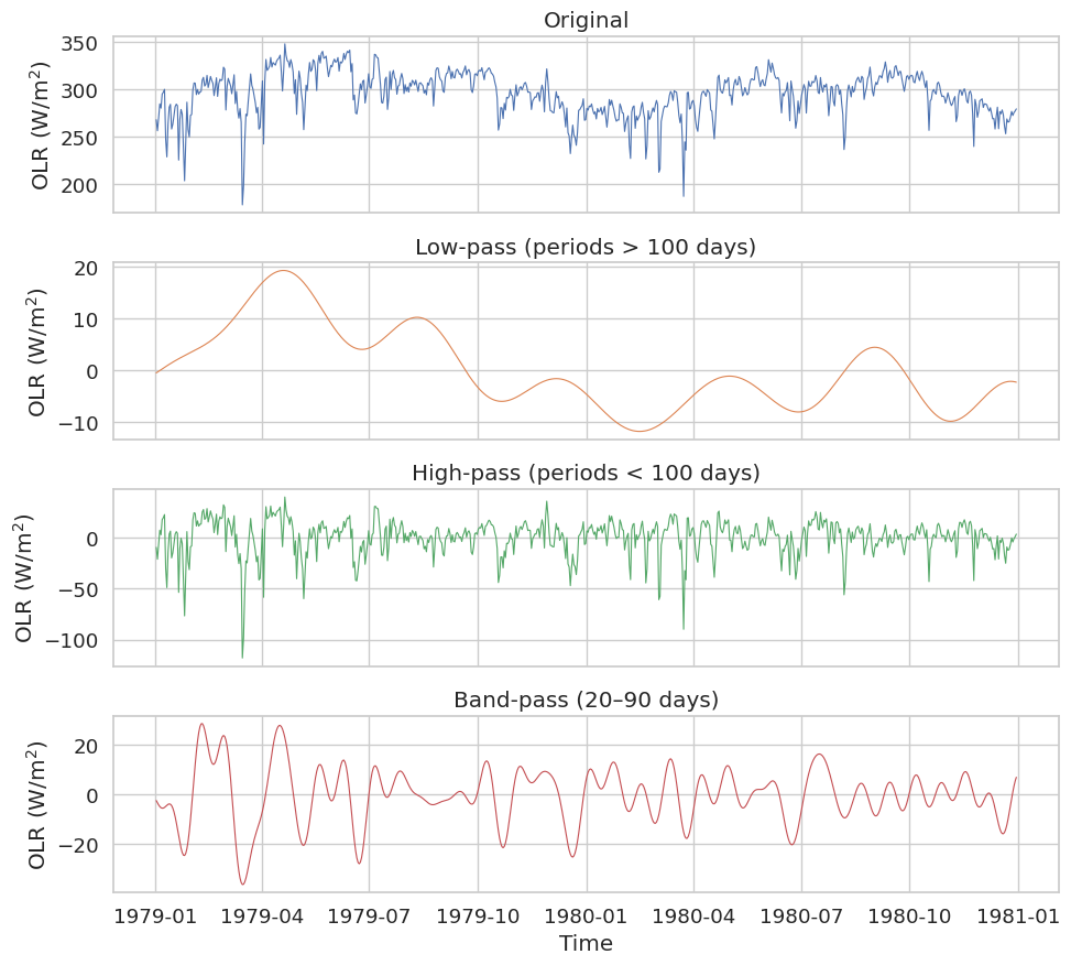

fig, ax = plt.subplots(figsize=(8, 4))
for filtered, label in [
    (lowpass, f"Low-pass (> {cutoff} d)"),
    (highpass, f"High-pass (< {cutoff} d)"),
    (bandpass, f"Band-pass ({bp_low}–{bp_high} d)"),
]:
    p, pv, _ = power_spectrum(filtered)
    ax.plot(p, pv, label=label, linewidth=1.6)

ax.set_xscale("log")
ax.set_xlim(10, n_time)
ax.set_xlabel("Period (days)")
ax.set_ylabel("Explained variance (%)")
ax.set_title("Power spectra after filtering")
ax.legend()
plt.show()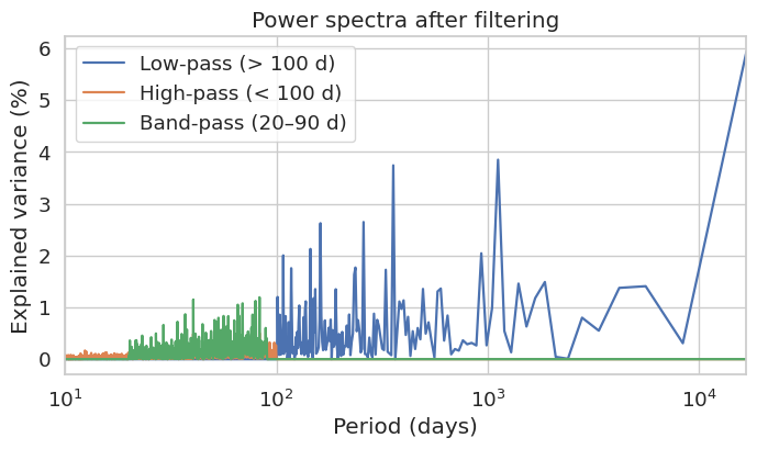

Summary¶

The power spectrum of a single-pixel time series reveals which time scales carry the most variance, often the annual cycle at ~365 days. Spectral filters multiply the Fourier coefficients by a mask: low-pass keeps slow variations, high-pass keeps fast ones, and band-pass targets a range such as 20–90 days for intraseasonal studies Zhang, 2013.

What’s next?¶

Spectral filtering works cleanly when the signal is smooth, but real climate series often contain sharp transitions and finite-record edges that the Fourier basis struggles to represent. The next notebook, Limitation of the Fourier transform and Fourier series: The Gibbs Phenomenon, illustrates how partial Fourier sums overshoot near discontinuities, a caveat to keep in mind whenever interpreting filtered time series or truncated spectra.

References¶

Lee, H.-T., & others. (2014). NOAA climate data record (CDR) of daily outgoing longwave radiation (OLR), version 1.2. (No Title).
Zhang, C. (2013). Madden–Julian oscillation: Bridging weather and climate. Bulletin of the American Meteorological Society, 94(12), 1849–1870.