SP2 Plots For SAIL events

---

Overview

This notebook will introduce the basics of gridded, labeled data with Xarray. Since Xarray introduces additional abstractions on top of plain arrays of data, our goal is to show why these abstractions are useful and how they frequently lead to simpler, more robust code.

We’ll cover these topics:

1. Create a DataArray, one of the core object types in Xarray

2. Understand how to use named coordinates and metadata in a DataArray

3. Combine individual DataArrays into a Dataset, the other core object type in Xarray

4. Subset, slice, and interpolate the data using named coordinates

5. Open netCDF data using XArray

6. Basic subsetting and aggregation of a Dataset

7. Brief introduction to plotting with Xarray

Prerequisites

Concepts	Importance	Notes
NumPy Basics	Necessary
Intermediate NumPy	Helpful	Familiarity with indexing and slicing arrays
NumPy Broadcasting	Helpful	Familiar with array arithmetic and broadcasting
Introduction to Pandas	Helpful	Familiarity with labeled data
Datetime	Helpful	Familiarity with time formats and the timedelta object
Understanding of NetCDF	Helpful	Familiarity with metadata structure

• Time to learn: 30 minutes

---

Imports

Simmilar to numpy, np; pandas, pd; you may often encounter xarray imported within a shortened namespace as xr.

import act
import numpy as np
import xarray as xr
import matplotlib.pyplot as plt

Introducing the DataArray and Dataset

Xarray expands on the capabilities on NumPy arrays, providing a lot of streamlined data manipulation. It is similar in that respect to Pandas, but whereas Pandas excels at working with tabular data, Xarray is focused on N-dimensional arrays of data (i.e. grids). Its interface is based largely on the netCDF data model (variables, attributes, and dimensions), but it goes beyond the traditional netCDF interfaces to provide functionality similar to netCDF-java’s Common Data Model (CDM).

For event #1 Jan2-7 2022

###For Event #3

# Set your username and token here!
username = 'adriancortessantos'
token = '<https://adc.arm.gov/armlive/livedata/home>`_.'

# Set the datastream and start/enddates
datastream = 'gucaossp2bc60sS2.b1'
startdate = '2022-01-02'
enddate = '2022-01-08'

# Use ACT to easily download the data.  Watch for the data citation!  Show some support
# for ARM's instrument experts and cite their data if you use it in a publication
result = act.discovery.download_arm_data(username, token, datastream, startdate, enddate)
ds_sp2 = act.io.read_arm_netcdf(result)

[DOWNLOADING] gucaossp2bc60sS2.b1.20220102.000000.nc
[DOWNLOADING] gucaossp2bc60sS2.b1.20220103.000000.nc
[DOWNLOADING] gucaossp2bc60sS2.b1.20220104.000000.nc
[DOWNLOADING] gucaossp2bc60sS2.b1.20220105.000000.nc
[DOWNLOADING] gucaossp2bc60sS2.b1.20220106.000000.nc
[DOWNLOADING] gucaossp2bc60sS2.b1.20220107.000000.nc

If you use these data to prepare a publication, please cite:

Jackson, R., Sedlacek, A., Salwen, C., & Hayes, C. Single Particle Soot
Photometer (AOSSP2BC60S). Atmospheric Radiation Measurement (ARM) User Facility.
https://doi.org/10.5439/1807910

print(ds_sp2)

<xarray.Dataset> Size: 68MB
Dimensions:       (time: 14160, bound: 2, bin: 199)
Coordinates:
  * time          (time) datetime64[ns] 113kB 2022-01-20T00:00:00.617000 ... ...
  * bin           (bin) float64 2kB 0.0125 0.0175 0.0225 ... 0.9925 0.9975 1.002
Dimensions without coordinates: bound
Data variables:
    base_time     (time) datetime64[ns] 113kB 2022-01-20 ... 2022-01-29
    time_offset   (time) datetime64[ns] 113kB 2022-01-20T00:00:00.617000 ... ...
    time_bounds   (time, bound) object 227kB dask.array<chunksize=(1416, 2), meta=np.ndarray>
    bin_bounds    (time, bin, bound) float64 45MB dask.array<chunksize=(1416, 199, 2), meta=np.ndarray>
    sp2_rbc_conc  (time) float64 113kB dask.array<chunksize=(1416,), meta=np.ndarray>
    sp2_cnts      (time, bin) float64 23MB dask.array<chunksize=(1416, 199), meta=np.ndarray>
    lat           (time) float32 57kB 38.9 38.9 38.9 38.9 ... 38.9 38.9 38.9
    lon           (time) float32 57kB -106.9 -106.9 -106.9 ... -106.9 -106.9
    alt           (time) float32 57kB 3.137e+03 3.137e+03 ... 3.137e+03
Attributes: (12/19)
    command_line:          aossp2bc60s --max-runtime 0 -s guc -f S2
    Conventions:           ARM-1.3
    process_version:       ingest-aossp2bc60s-1.1-0.el7
    dod_version:           aossp2bc60s-b1-1.0
    input_datastreams:     gucaossp2auxS2.a0 : 2.2 : 20220120.000000\ngucaoss...
    site_id:               guc
    ...                    ...
    processed_with:        PySP2 0.1.0
    history:               created by user dsmgr on machine procnode1 at 2022...
    _file_dates:           ['20220120', '20220121', '20220122', '20220123', '...
    _file_times:           ['000000', '000000', '000000', '000000', '000000',...
    _datastream:           gucaossp2bc60sS2.b1
    _arm_standards_flag:   1

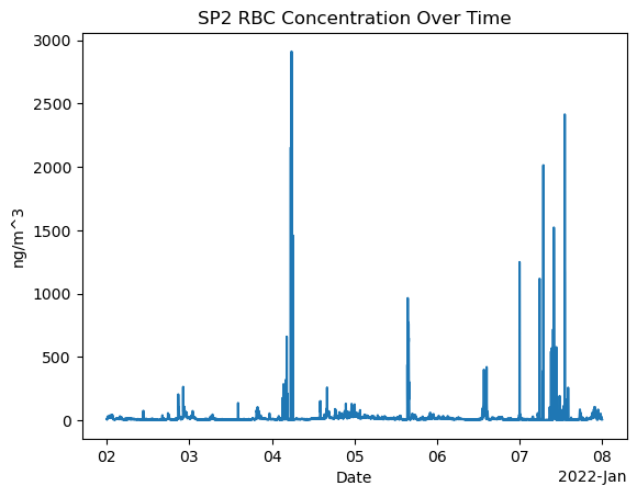
Plot rBc Concentration with xarray

import xarray as xr
import matplotlib.pyplot as plt


# Assuming you have already loaded your dataset as sp2_ds
# Plot the sp2_rbc_conc over time
ds_sp2['sp2_rbc_conc'].plot()
plt.title('SP2 RBC Concentration Over Time')
plt.xlabel('Date')
plt.ylabel('ng/m^3')
plt.show()

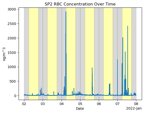
Apply Date-night highlight

import xarray as xr
import matplotlib.pyplot as plt

# Assuming you have already loaded your dataset as sp2_ds
# Plot the sp2_rbc_conc over time
fig, ax = plt.subplots()
ds_sp2['sp2_rbc_conc'].plot(ax=ax)
ax.set_title('SP2 RBC Concentration Over Time')
ax.set_xlabel('Date')
ax.set_ylabel('ng/m^3')

# Define day and night periods (assuming 6 AM to 6 PM as day)
day_start = 6   # 6 AM
day_end = 18    # 6 PM

# Shade periods for each day in the dataset
date_range = pd.date_range(ds_sp2['time'].min().values, ds_sp2['time'].max().values, freq='D')

for date in date_range:
    # Night period before day start
    ax.axvspan(date, date + pd.Timedelta(hours=day_start), color='grey', alpha=0.3)
    # Day period
    ax.axvspan(date + pd.Timedelta(hours=day_start), date + pd.Timedelta(hours=day_end), color='yellow', alpha=0.3)
    # Night period after day end
    ax.axvspan(date + pd.Timedelta(hours=day_end), date + pd.Timedelta(hours=24), color='grey', alpha=0.3)

plt.show()

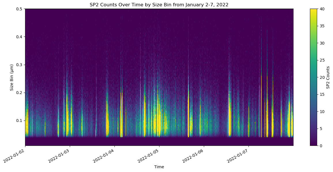
import xarray as xr
import matplotlib.pyplot as plt
import numpy as np

# Assuming 'ds_sp2' is already loaded and 'sp2_cnts' is computed
sp2_cnts = ds_sp2['sp2_cnts'].compute()

# Convert 'time' to a regular NumPy array of datetime objects for compatibility
times = ds_sp2['time'].values
bins = ds_sp2['bin'].values

# Filter bins and sp2_cnts for bins <= 0.6 micrometers
mask = bins <= 0.5
filtered_bins = bins[mask]
filtered_sp2_cnts = sp2_cnts[:, mask]

# Create the plot
fig, ax = plt.subplots(figsize=(15, 7))
# Use meshgrid to create 2D grid coordinates for times and filtered bins, necessary for pcolormesh
T, B = np.meshgrid(times, filtered_bins)
# Plot with specified color scale range
c = ax.pcolormesh(T, B, filtered_sp2_cnts.T, shading='auto', vmin=0, vmax=40)  # Set color scale limits here

# Adding a colorbar to represent the concentration scales
cbar = plt.colorbar(c, ax=ax)
cbar.set_label('SP2 Counts')

# Customization of the plot
ax.set_title('SP2 Counts Over Time by Size Bin from January 2-7, 2022')
ax.set_xlabel('Time')
ax.set_ylabel('Size Bin (μm)')

# Format x-axis to handle datetime objects nicely
plt.gcf().autofmt_xdate()  # Auto format date labels

plt.show()

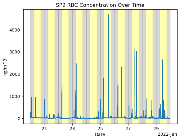
For Event 2 Jan 20-30

# Set your username and token here!
username = 'adriancortessantos'
token = '<https://adc.arm.gov/armlive/livedata/home>`_.'

# Set the datastream and start/enddates
datastream = 'gucaossp2bc60sS2.b1'
startdate = '2022-01-20'
enddate = '2022-01-30'

# Use ACT to easily download the data.  Watch for the data citation!  Show some support
# for ARM's instrument experts and cite their data if you use it in a publication
result = act.discovery.download_arm_data(username, token, datastream, startdate, enddate)
ds_sp2 = act.io.read_arm_netcdf(result)

[DOWNLOADING] gucaossp2bc60sS2.b1.20220120.000000.nc
[DOWNLOADING] gucaossp2bc60sS2.b1.20220122.000000.nc
[DOWNLOADING] gucaossp2bc60sS2.b1.20220121.000000.nc
[DOWNLOADING] gucaossp2bc60sS2.b1.20220124.000000.nc
[DOWNLOADING] gucaossp2bc60sS2.b1.20220123.000000.nc
[DOWNLOADING] gucaossp2bc60sS2.b1.20220128.000000.nc
[DOWNLOADING] gucaossp2bc60sS2.b1.20220125.000000.nc
[DOWNLOADING] gucaossp2bc60sS2.b1.20220126.000000.nc
[DOWNLOADING] gucaossp2bc60sS2.b1.20220127.000000.nc
[DOWNLOADING] gucaossp2bc60sS2.b1.20220129.000000.nc

If you use these data to prepare a publication, please cite:

Jackson, R., Sedlacek, A., Salwen, C., & Hayes, C. Single Particle Soot
Photometer (AOSSP2BC60S). Atmospheric Radiation Measurement (ARM) User Facility.
https://doi.org/10.5439/1807910

import xarray as xr
import matplotlib.pyplot as plt

# Assuming you have already loaded your dataset as sp2_ds
# Plot the sp2_rbc_conc over time
fig, ax = plt.subplots()
ds_sp2['sp2_rbc_conc'].plot(ax=ax)
ax.set_title('SP2 RBC Concentration Over Time')
ax.set_xlabel('Date')
ax.set_ylabel('ng/m^3')

# Define day and night periods (assuming 6 AM to 6 PM as day)
day_start = 6   # 6 AM
day_end = 18    # 6 PM

# Shade periods for each day in the dataset
date_range = pd.date_range(ds_sp2['time'].min().values, ds_sp2['time'].max().values, freq='D')

for date in date_range:
    # Night period before day start
    ax.axvspan(date, date + pd.Timedelta(hours=day_start), color='grey', alpha=0.3)
    # Day period
    ax.axvspan(date + pd.Timedelta(hours=day_start), date + pd.Timedelta(hours=day_end), color='yellow', alpha=0.3)
    # Night period after day end
    ax.axvspan(date + pd.Timedelta(hours=day_end), date + pd.Timedelta(hours=24), color='grey', alpha=0.3)

plt.show()

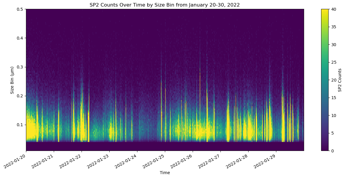
import xarray as xr
import matplotlib.pyplot as plt
import numpy as np

# Assuming 'ds_sp2' is already loaded and 'sp2_cnts' is computed
sp2_cnts = ds_sp2['sp2_cnts'].compute()

# Convert 'time' to a regular NumPy array of datetime objects for compatibility
times = ds_sp2['time'].values
bins = ds_sp2['bin'].values

# Filter bins and sp2_cnts for bins <= 0.6 micrometers
mask = bins <= 0.5
filtered_bins = bins[mask]
filtered_sp2_cnts = sp2_cnts[:, mask]

# Create the plot
fig, ax = plt.subplots(figsize=(15, 7))
# Use meshgrid to create 2D grid coordinates for times and filtered bins, necessary for pcolormesh
T, B = np.meshgrid(times, filtered_bins)
# Plot with specified color scale range
c = ax.pcolormesh(T, B, filtered_sp2_cnts.T, shading='auto', vmin=0, vmax=40)  # Set color scale limits here

# Adding a colorbar to represent the concentration scales
cbar = plt.colorbar(c, ax=ax)
cbar.set_label('SP2 Counts')

# Customization of the plot
ax.set_title('SP2 Counts Over Time by Size Bin from January 20-30, 2022')
ax.set_xlabel('Time')
ax.set_ylabel('Size Bin (μm)')

# Format x-axis to handle datetime objects nicely
plt.gcf().autofmt_xdate()  # Auto format date labels

plt.show()

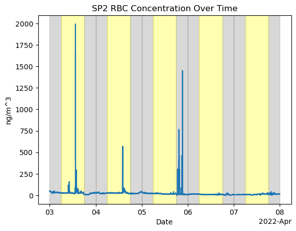
For event 3 Apr3-8 2022

# Set your username and token here!
username = 'adriancortessantos'
token = '<https://adc.arm.gov/armlive/livedata/home>`_.'

# Set the datastream and start/enddates
datastream = 'gucaossp2bc60sS2.b1'
startdate = '2022-04-03'
enddate = '2022-04-08'


# Use ACT to easily download the data.  Watch for the data citation!  Show some support
# for ARM's instrument experts and cite their data if you use it in a publication
result = act.discovery.download_arm_data(username, token, datastream, startdate, enddate)
ds_sp2 = act.io.read_arm_netcdf(result)

[DOWNLOADING] gucaossp2bc60sS2.b1.20220403.000000.nc
[DOWNLOADING] gucaossp2bc60sS2.b1.20220406.000000.nc
[DOWNLOADING] gucaossp2bc60sS2.b1.20220404.000000.nc
[DOWNLOADING] gucaossp2bc60sS2.b1.20220405.000000.nc
[DOWNLOADING] gucaossp2bc60sS2.b1.20220407.000000.nc

If you use these data to prepare a publication, please cite:

Jackson, R., Sedlacek, A., Salwen, C., & Hayes, C. Single Particle Soot
Photometer (AOSSP2BC60S). Atmospheric Radiation Measurement (ARM) User Facility.
https://doi.org/10.5439/1807910

import xarray as xr
import matplotlib.pyplot as plt

# Assuming you have already loaded your dataset as sp2_ds
# Plot the sp2_rbc_conc over time
fig, ax = plt.subplots()
ds_sp2['sp2_rbc_conc'].plot(ax=ax)
ax.set_title('SP2 RBC Concentration Over Time')
ax.set_xlabel('Date')
ax.set_ylabel('ng/m^3')

# Define day and night periods (assuming 6 AM to 6 PM as day)
day_start = 6   # 6 AM
day_end = 18    # 6 PM

# Shade periods for each day in the dataset
date_range = pd.date_range(ds_sp2['time'].min().values, ds_sp2['time'].max().values, freq='D')

for date in date_range:
    # Night period before day start
    ax.axvspan(date, date + pd.Timedelta(hours=day_start), color='grey', alpha=0.3)
    # Day period
    ax.axvspan(date + pd.Timedelta(hours=day_start), date + pd.Timedelta(hours=day_end), color='yellow', alpha=0.3)
    # Night period after day end
    ax.axvspan(date + pd.Timedelta(hours=day_end), date + pd.Timedelta(hours=24), color='grey', alpha=0.3)

plt.show()

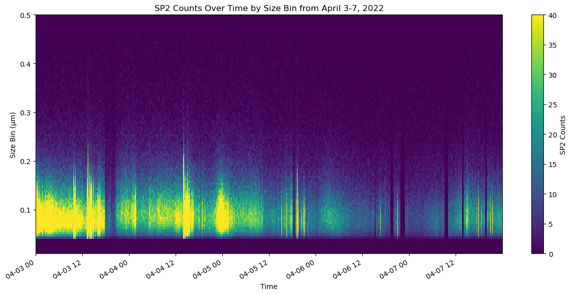
import xarray as xr
import matplotlib.pyplot as plt
import numpy as np

# Assuming 'ds_sp2' is already loaded and 'sp2_cnts' is computed
sp2_cnts = ds_sp2['sp2_cnts'].compute()

# Convert 'time' to a regular NumPy array of datetime objects for compatibility
times = ds_sp2['time'].values
bins = ds_sp2['bin'].values

# Filter bins and sp2_cnts for bins <= 0.6 micrometers
mask = bins <= 0.5
filtered_bins = bins[mask]
filtered_sp2_cnts = sp2_cnts[:, mask]

# Create the plot
fig, ax = plt.subplots(figsize=(15, 7))
# Use meshgrid to create 2D grid coordinates for times and filtered bins, necessary for pcolormesh
T, B = np.meshgrid(times, filtered_bins)
# Plot with specified color scale range
c = ax.pcolormesh(T, B, filtered_sp2_cnts.T, shading='auto', vmin=0, vmax=40)  # Set color scale limits here

# Adding a colorbar to represent the concentration scales
cbar = plt.colorbar(c, ax=ax)
cbar.set_label('SP2 Counts')

# Customization of the plot
ax.set_title('SP2 Counts Over Time by Size Bin from April 3-7, 2022')
ax.set_xlabel('Time')
ax.set_ylabel('Size Bin (μm)')

# Format x-axis to handle datetime objects nicely
plt.gcf().autofmt_xdate()  # Auto format date labels

plt.show()