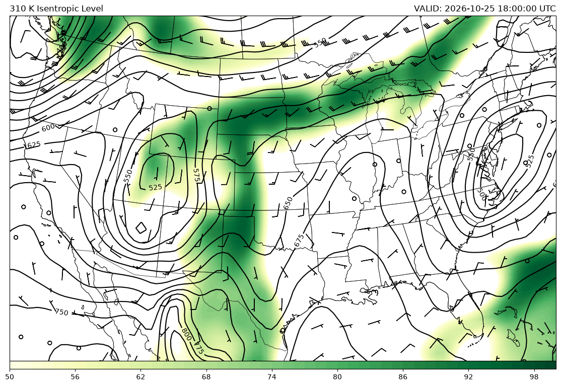
Isentropic Analysis - The MetPy Cookbook

The MetPy function metpy.calc.isentropic_interpolation allows for isentropic analysis from model analysis data in isobaric coordinates.

from datetime import datetime, timedelta

import cartopy.crs as ccrs
import cartopy.feature as cfeature
import matplotlib.pyplot as plt
import metpy.calc as mpcalc
from metpy.units import units
import numpy as np
from siphon.catalog import TDSCatalog
from xarray.backends import NetCDF4DataStore
import xarray as xr

Getting the data

In this example, the latest GFS forecasts data from the National Centers for Environmental Information (https://www.ncei.noaa.gov) will be used, courtesy of the Univeristy Corporation for Atmospheric Research Thredds Data Server.

# Latest GFS Dataset
cat = TDSCatalog('http://thredds.ucar.edu/thredds/catalog/grib/'
                 'NCEP/GFS/Global_0p5deg/catalog.xml')
ncss = cat.latest.subset()

# Find the start of the model run and define time range
start_time = ncss.metadata.time_span['begin']
start = datetime.strptime(start_time, '%Y-%m-%dT%H:%M:%Sz')
end = start + timedelta(hours=9)

# Query for Latest GFS Run
gfsdata = ncss.query().time_range(start, end).accept('netcdf4')

gfsdata.variables('Temperature_isobaric',
                  'u-component_of_wind_isobaric',
                  'v-component_of_wind_isobaric',
                  'Relative_humidity_isobaric').add_lonlat()

# Set the lat/lon box for the data you want to pull in.
# lonlat_box(north_lat,south_lat,east_lon,west_lon)
gfsdata.lonlat_box(-150, -50, 15, 65)

# Actually getting the data
data = ncss.get_data(gfsdata)

# Make into an xarray Dataset object
ds = xr.open_dataset(NetCDF4DataStore(data)).metpy.parse_cf()

dlev_hght = ds.Temperature_isobaric.dims[1]
dlev_uwnd = ds['u-component_of_wind_isobaric'].dims[1]
lat = ds.latitude
lon = ds.longitude

lev_hght = ds[dlev_hght]
lev_uwnd = ds[dlev_uwnd]

# Due to a different number of vertical levels find where they are common
_, _, common_ind = np.intersect1d(lev_uwnd, lev_hght, return_indices=True)

common_levels = lev_hght[common_ind].metpy.unit_array
times = ds.Temperature_isobaric.metpy.time
vtimes = times.values.astype('datetime64[ms]').astype('O')
temps = ds.Temperature_isobaric.metpy.unit_array
uwnd = ds['u-component_of_wind_isobaric'].metpy.unit_array
vwnd = ds['v-component_of_wind_isobaric'].metpy.unit_array
relh = ds.Relative_humidity_isobaric.metpy.unit_array

To properly interpolate to isentropic coordinates, the function must know the desired output isentropic levels. An array with these levels will be created below.

isentlevs = np.arange(310, 316, 5) * units.kelvin

Conversion to Isentropic Coordinates

Once model data in isobaric coordinates has been pulled and the desired isentropic levels created, the conversion to isentropic coordinates can begin. Data will be passed to the function as below. The function requires that isentropic levels, isobaric levels, and temperature be input. Any additional inputs (in this case relative humidity, u, and v wind components) will be linearly interpolated to isentropic space.

isent_anal = mpcalc.isentropic_interpolation(isentlevs,
                                             common_levels,
                                             temps[:, common_ind, :, :],
                                             relh,
                                             uwnd,
                                             vwnd,
                                             vertical_dim=1)

/tmp/ipykernel_4390/414936893.py:1: UserWarning: Interpolation point out of data bounds encountered
  isent_anal = mpcalc.isentropic_interpolation(isentlevs,

The output is a list, so now we will separate the variables to different names before plotting.

isentprs, isentrh, isentu, isentv = isent_anal

A quick look at the shape of these variables will show that the data is now in isentropic coordinates, with the number of vertical levels as specified above.

print(isentprs.shape)
print(isentrh.shape)
print(isentu.shape)
print(isentv.shape)

(4, 2, 101, 201)
(4, 2, 101, 201)
(4, 2, 101, 201)
(4, 2, 101, 201)

Plotting the Isentropic Analysis

Set up our projection

crs = ccrs.LambertConformal(central_longitude=-100.0, central_latitude=45.0)

# Set up our array of latitude and longitude values and transform to
# the desired projection.
clons, clats = np.meshgrid(lon, lat)

# Get data to plot state and province boundaries
states_provinces = cfeature.NaturalEarthFeature(
    category='cultural',
    name='admin_1_states_provinces_lakes',
    scale='50m',
    facecolor='none')

# Choose Isentropic Level index value
level = 0 # [310, 315]

# Choose forecast hour index value
FH = 0 # [0, 3, 6, 9]

# Start Figure
fig = plt.figure(1, figsize=(14., 12.))
ax = plt.subplot(111, projection=crs)

# Set plot extent
ax.set_extent((-121., -74., 25., 50.), crs=ccrs.PlateCarree())
ax.coastlines('50m', edgecolor='black', linewidth=0.75)
ax.add_feature(states_provinces, edgecolor='black', linewidth=0.5)

# Plot the 300K surface
clevisent = np.arange(0, 1000, 25)
cs = ax.contour(clons, clats,
                mpcalc.smooth_n_point(isentprs[FH, level, :, :], 9, 4),
                clevisent,
                transform=ccrs.PlateCarree(),
                colors='k', linewidths=1.5, linestyles='solid')
plt.clabel(cs, fontsize=10, inline=1, inline_spacing=7,
           fmt='%i', rightside_up=True, use_clabeltext=True)

cf = ax.contourf(clons, clats,
                 mpcalc.smooth_n_point(isentrh[FH, level, :, :], 9, 4),
                 np.arange(50, 101, 1),
                 transform=ccrs.PlateCarree(),
                 cmap=plt.cm.YlGn)
plt.colorbar(cf, orientation='horizontal', aspect=65, pad=0, extendrect='True')

wind_slice = (FH, level, slice(None, None, 5), slice(None, None, 5))
ax.barbs(clons[wind_slice[2:]], clats[wind_slice[2:]],
         isentu[wind_slice].m, isentv[wind_slice].m, length=6,
         transform=ccrs.PlateCarree())

# Make some titles
plt.title(f'{isentlevs[level].m:.0f} K Isentropic Level', loc='left')
plt.title(f'VALID: {vtimes[FH]} UTC', loc='right')