Multivariate EOFs: Extracting the MJO Signal - A Simple RMM-like Index - Spectral Analysis for Geophysical Data Cookbook

Overview¶

Standard EOF analysis decomposes a single space–time field into orthogonal patterns of variability. Multivariate EOF analysis extends the same idea to several variables at once: the fields are stacked side by side into a single data matrix, so that the leading modes describe variability that is coherent across all variables simultaneously.

As a worked example we apply the method to tropical OLR and zonal wind at 850 and 200 hPa, the same combination used by Wheeler & Hendon (2004) to construct the RMM index that monitors the Madden–Julian Oscillation (MJO).

Why combine variables before doing EOFs
Load and preprocess the three input fields
Build and normalize the combined data matrix
Compute the EOFs and principal components
Interpret the leading pair as a coupled mode

Prerequisites¶

Concepts	Importance	Notes
3D EOFs	Necessary	Covariance, eigen-decomposition, PCs vs EOF maps
Extended EOFs	Helpful	Same workflow on real geophysical data
Harmonic anomalies	Helpful	Seasonal cycle removal

Time to learn: 30 min

Imports¶

import numpy as np
import xarray as xr
import matplotlib.pyplot as plt
import seaborn as sns
import s3fs

sns.set_theme(style="whitegrid", context="notebook", font_scale=1.2)

The multivariate EOF idea¶

Recall from 3D EOFs that EOF analysis arranges a field in a matrix $\mathbf{X} \in \mathbb{R}^{n_t \times m}$ (rows are times, columns are spatial points) and diagonalizes its covariance matrix.

For $V$ variables, each producing its own matrix $\mathbf{X}^{(v)} \in \mathbb{R}^{n_t \times m_v}$ , we horizontally concatenate them after normalizing each field so that no single variable dominates the variance:

\mathbf{X} = \bigl[\mathbf{X}^{(1)} \;\big|\; \mathbf{X}^{(2)} \;\big|\; \cdots \;\big|\; \mathbf{X}^{(V)}\bigr] \in \mathbb{R}^{n_t \times \sum_v m_v}

(1)

The eigen-decomposition is then performed on the combined matrix exactly as in the single-variable case. Each EOF is a long vector that, once split back into its $V$ blocks, gives the spatial structure of every variable in the mode. The associated principal component (PC) describes how strongly this multi-variable pattern is expressed at each time.

Load the input data¶

We use the same Pythia cloud Zarr datasets as the other notebooks: NOAA OLR Lee & others, 2014 and NCEP/NCAR zonal wind at 850 and 200 hPa Kanamitsu et al., 2002.

URL = "https://js2.jetstream-cloud.org:8001/"
fs = s3fs.S3FileSystem(anon=True, client_kwargs=dict(endpoint_url=URL))

olr = (
    xr.open_zarr(s3fs.S3Map(root="pythia/olr_noaa.zarr", s3=fs, check=False))
    .rename_vars({"__xarray_dataarray_variable__": "olr"})["olr"]
)

uwind = xr.open_zarr(s3fs.S3Map(root="pythia/uwind-ncep-ncar.zarr", s3=fs, check=False))
u850 = uwind["uwnd"].isel(level=0, drop=True)
u200 = uwind["uwnd"].isel(level=1, drop=True)

Preprocessing¶

A few short steps prepare the data for EOF analysis:

Align time stamps to daily resolution and select a common period.
Restrict each field to the equatorial band (15°S–15°N) and fill short time gaps by linear interpolation.
Remove the seasonal cycle by least-squares fitting the first 4 harmonics of the annual cycle and subtracting the fit (see Remove the seasonal cycle using harmonic regression).
Take a cosine-weighted latitude mean over 15°S–15°N so each field becomes a (time, lon) array.
Remove variability slower than the MJO time scale by subtracting a 120-day running mean. This keeps the leading EOFs focused on intraseasonal variability rather than ENSO.

def remove_seasonal_cycle_harmonic(data, n_harmonics=4, year_period=365.25):
    """Subtract the first ``n_harmonics`` of the annual cycle along the leading (time) axis."""
    n_time = data.shape[0]
    t = np.arange(n_time)

    X = np.ones((n_time, 2 * n_harmonics + 1))
    for k in range(1, n_harmonics + 1):
        X[:, 2 * k - 1] = np.sin(k * 2 * np.pi * t / year_period)
        X[:, 2 * k] = np.cos(k * 2 * np.pi * t / year_period)

    data_2d = data.reshape(n_time, -1)
    coeffs = np.linalg.lstsq(X, data_2d, rcond=None)[0]
    anomalies = data_2d - X @ coeffs
    return anomalies.reshape(data.shape)


def preprocess(da, start="1979-01-01", end="2024-12-31",
               lat_bounds=(-15, 15), lowfreq_window=120, n_harmonics=4):
    da = da.assign_coords(time=da["time"].dt.floor("D"))
    if bool(da["lon"].min() < 0):
        da = da.assign_coords(lon=(da["lon"] % 360)).sortby("lon")

    da = da.sel(time=slice(start, end))

    lat_descending = bool(da["lat"][0] > da["lat"][-1])
    lat_slice = slice(*sorted(lat_bounds, reverse=lat_descending))
    da = da.sel(lat=lat_slice).load()
    da = da.interpolate_na(dim="time", method="linear")

    anom = xr.DataArray(
        remove_seasonal_cycle_harmonic(da.values, n_harmonics=n_harmonics),
        coords=da.coords,
        dims=da.dims,
        name=da.name,
    )

    weights = np.cos(np.deg2rad(anom["lat"]))
    anom = anom.weighted(weights).mean(dim="lat")

    low_freq = anom.rolling(time=lowfreq_window, min_periods=lowfreq_window).mean()
    return (anom - low_freq).dropna(dim="time")

olr_anom = preprocess(olr)
u850_anom = preprocess(u850)
u200_anom = preprocess(u200)

olr_anom, u850_anom, u200_anom = xr.align(olr_anom, u850_anom, u200_anom, join="inner")
olr_anom.shape

(16683, 144)

Build the combined matrix¶

Each field is divided by its global standard deviation so the three variables contribute on comparable scales. We then concatenate them along the spatial dimension.

def normalize(da):
    return (da - da.mean()) / da.std()

fields = [normalize(da).transpose("time", "lon").values
          for da in (olr_anom, u850_anom, u200_anom)]

X = np.concatenate(fields, axis=1).astype(np.float32)
X -= X.mean(axis=0, keepdims=True)

n_time, n_features = X.shape
n_lon = olr_anom.sizes["lon"]
print(f"Combined matrix: {n_time} times × {n_features} features ({n_lon} longitudes × 3 variables)")

Combined matrix: 16683 times × 432 features (144 longitudes × 3 variables)

Thus it is simpler to used the 432x432 matrix for the EOF

EOF analysis¶

We follow the same workflow as in 3D EOFs: form the spatial covariance matrix $\mathbf{C} = \mathbf{X}^{\mathsf T}\mathbf{X}/(n_t-1)$ , solve the eigenvalue problem with numpy.linalg.eigh, and obtain the PCs by projecting the data onto each eigenvector.

C = (X.T @ X) / (n_time - 1)
eigvals, eigvecs = np.linalg.eigh(C)

order = np.argsort(eigvals)[::-1]
eigvals = eigvals[order]
eigvecs = eigvecs[:, order]

explained_variance = 100 * eigvals / eigvals.sum()
pcs = X @ eigvecs

pcs = pcs / pcs.std(axis=0, keepdims=True)
eofs = eigvecs.T * pcs.std(axis=0, keepdims=True).T

Explained variance¶

Because the matrix mixes three variables and all longitudes, individual modes capture only a modest share of the total variance. What matters is whether the leading modes stand out from the rest of the spectrum.

n_show = 10
fig, ax = plt.subplots(figsize=(7, 4))
ax.bar(np.arange(1, n_show + 1), explained_variance[:n_show])
ax.set_xlabel("Mode index $k$")
ax.set_ylabel("Explained variance [%]")
ax.set_title("Explained variance of leading multivariate EOFs")
ax.set_xticks(np.arange(1, n_show + 1));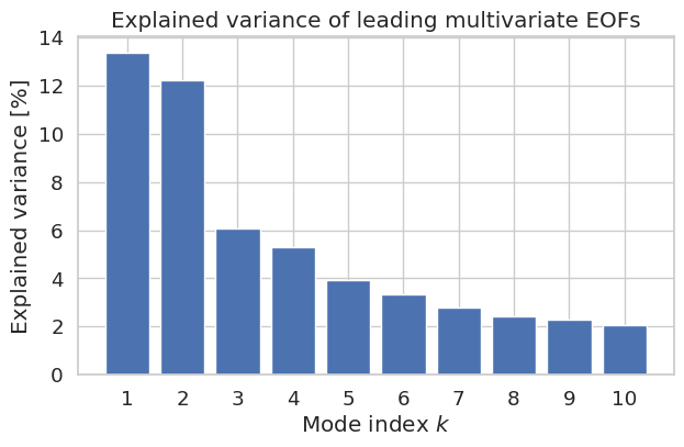

Spatial structure of the leading modes¶

Each EOF is a vector of length $3 \times n_{lon}$ . Splitting it back into three blocks recovers the longitude-dependent loading for OLR, U850, and U200 separately.

lon = olr_anom["lon"].values
blocks = {"OLR": slice(0, n_lon),
          "U850": slice(n_lon, 2 * n_lon),
          "U200": slice(2 * n_lon, 3 * n_lon)}

fig, axes = plt.subplots(2, 1, figsize=(10, 6), sharex=True)
for ax, k in zip(axes, [0, 1]):
    for name, sl in blocks.items():
        ax.plot(lon, eofs[k, sl], lw=2, label=name)
    ax.axhline(0, color="k", lw=0.8)
    ax.set_title(f"EOF {k+1} [Exp Var: {explained_variance[k]:.1f}%]")
    ax.set_ylabel("Loading")
    ax.legend(loc="upper right")
    ax.set_xlim(0, 360)
axes[-1].set_xlabel("Longitude [°E]")
plt.tight_layout()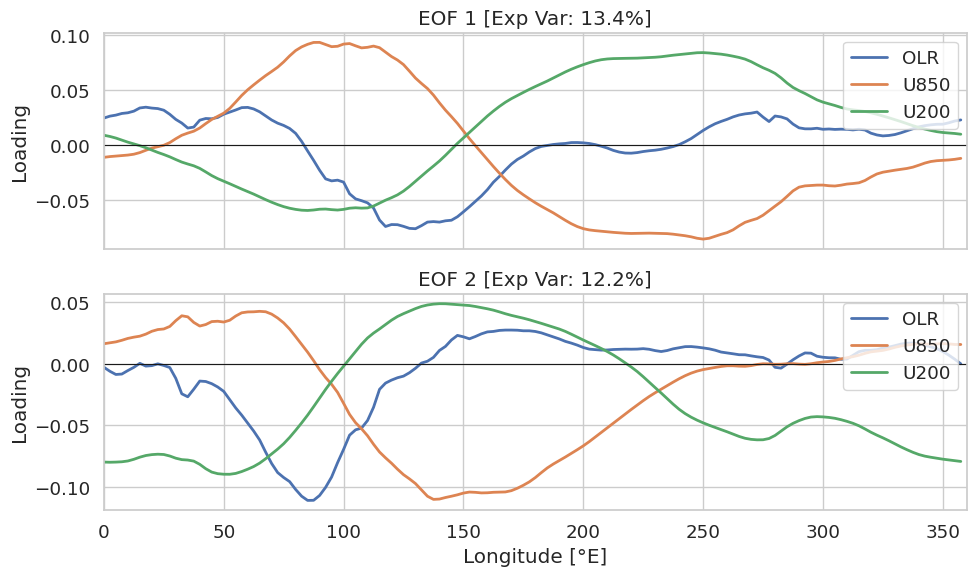

The result mirrors Fig. 1 of Wheeler & Hendon (2004). EOFs 1 and 2 have similar amplitudes but their convective centres are shifted in longitude. As discussed in 3D EOFs, a pair of modes with comparable variance and a spatial quadrature relationship is the signature of a propagating signal, here, the eastward-moving convective envelope of the MJO.

Principal component time series¶

The standardized PCs describe how strongly each EOF pattern projects onto the data at each day. We show a short window so the intraseasonal character is visible.

time = olr_anom["time"].values
pc_ds = xr.Dataset(
    {f"PC{k+1}": ("time", pcs[:, k]) for k in range(3)},
    coords={"time": time},
)

fig, ax = plt.subplots(figsize=(12, 4))
pc_ds["PC1"].sel(time=slice("2001", "2002")).plot(
    ax=ax, lw=1.2, label="PC1")
pc_ds["PC2"].sel(time=slice("2001", "2002")).plot(
    ax=ax, lw=1.2, label="PC2")
ax.axhline(0, color="k", lw=0.8)
ax.set_title("Standardized PC1 and PC2 (2001-2002)")
ax.set_ylabel("PC amplitude")
ax.legend()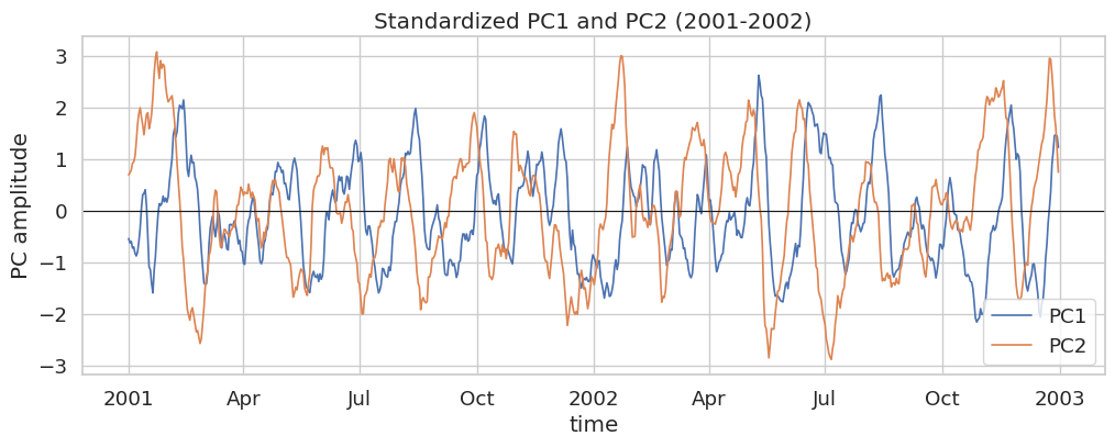

Validation: variance in the MJO band¶

If the leading pair really captures MJO-like variability, most of its spectral power should lie in the 20–90 day band Zhang, 2013 identified by Wheeler & Hendon (2004). A simple periodogram of each PC is enough to check this.

from scipy.signal import periodogram

def band_fraction(pc, band=(20, 90)):
    freq, psd = periodogram(pc - pc.mean(), fs=1.0)
    freq, psd = freq[1:], psd[1:]
    period = 1 / freq
    mask = (period >= band[0]) & (period <= band[1])
    return np.trapezoid(psd[mask], freq[mask]) / np.trapezoid(psd, freq)

for k in range(3):
    f = band_fraction(pc_ds[f"PC{k+1}"].values)
    print(f"PC{k+1}: 20-90 day variance fraction = {f:.2%}")

PC1: 20-90 day variance fraction = 69.92%
PC2: 20-90 day variance fraction = 71.21%
PC3: 20-90 day variance fraction = 46.57%

PC1 and PC2 concentrate noticeably more of their variance in the MJO band than PC3, confirming that the multivariate EOF projection acts as a spatial filter for the coupled convection–circulation structure of the oscillation.

Summary¶

Multivariate EOF analysis is an extend of the standard EOF framework [3D EOFs] applied to a horizontally concatenated, per-variable normalized matrix.

The leading eigenvectors describe spatial patterns that vary coherently across all variables, and the associated PCs are time series of that joint variability

Using equatorial OLR, U850, and U200 as an example, the first two modes form a quadrature pair whose principal components concentrate variance at MJO intraseasonal periods, the same construction underlying the operational RMM index.

What’s next?¶

Regressing fields onto MJO indices: use PC1 and PC2 as predictors to build composite maps of related atmospheric fields.

References¶

Wheeler, M. C., & Hendon, H. H. (2004). An all-season real-time multivariate MJO index: Development of an index for monitoring and prediction. Monthly Weather Review, 132(8), 1917–1932.
Lee, H.-T., & others. (2014). NOAA climate data record (CDR) of daily outgoing longwave radiation (OLR), version 1.2. (No Title).
Kanamitsu, M., Ebisuzaki, W., Woollen, J., Yang, S.-K., Hnilo, J. J., Fiorino, M., & Potter, G. L. (2002). Ncep–doe amip-ii reanalysis (r-2). Bulletin of the American Meteorological Society, 83(11), 1631–1644.
Zhang, C. (2013). Madden–Julian oscillation: Bridging weather and climate. Bulletin of the American Meteorological Society, 94(12), 1849–1870.