Removing the Seasonal Cycle: Daily Climatology vs. Harmonic Regression - Spectral Analysis for Geophysical Data Cookbook

Overview¶

Before studying intraseasonal, interannual or other kinds of variability, we often remove the seasonal cycle to obtain anomalies, departures from the repeating annual pattern. This notebook compares two common approaches on daily 850-hPa zonal wind ( $u_{850}$ ) from the NCEP–NCAR Reanalysis Kanamitsu et al., 2002Kalnay et al., 2018 and inspects the resulting spectra.

We will:

Load daily $u_{850}$ from the public Pythia Zarr store.
Remove the seasonal cycle with daily climatology and harmonic regression.
Compare the fitted seasonal cycles, anomaly time series, spatial patterns of disagreement, and time-mean maps.
Resample to monthly means, compute monthly anomalies, and apply the FFT to see whether either method leaves residual seasonal power.

An anomaly is defined as

\text{anomaly} = \text{observed value} - \text{seasonal climatology}.

(1)

Prerequisites¶

Concepts	Importance	Notes
Remove the seasonal cycle using harmonic regression	Necessary	Harmonic design matrix and least-squares fit
The Discrete Fourier Transform	Helpful	Frequencies, periods, and Fourier coefficients
Fourier Power Spectrum and Spectral Filtering	Helpful	Power spectrum and explained variance

Time to learn: 25 minutes

Imports¶

All packages used in the rest of the notebook are imported up front. s3fs is configured to read anonymously from the public Pythia bucket on the Jetstream2 S3 endpoint. The Zarr store is read lazily with Dask; heavy array work runs in parallel only when we call dask.persist or .compute().

import dask

import numpy as np
import pandas as pd
import matplotlib.pyplot as plt
import seaborn as sns
import cartopy.crs as ccrs

import s3fs
import xarray as xr

sns.set_theme(style="whitegrid", context="notebook", font_scale=1.2)

URL = "https://js2.jetstream-cloud.org:8001/"
fs = s3fs.S3FileSystem(anon=True, client_kwargs=dict(endpoint_url=URL))

Load NCEP–NCAR zonal wind¶

We use daily 850-hPa zonal wind from the NCEP–NCAR Reanalysis Kanamitsu et al., 2002Kalnay et al., 2018, stored as a preprocessed Zarr dataset on the Pythia Jetstream2 bucket. The array stays lazy until we compute specific results.

For harmonic regression each latitude band needs the full time series and longitude, so we rechunk to {time: -1, lat: 10, lon: -1}. Dask can then parallelize the least-squares fit over latitude blocks. In this tutorial we are only to be analysing the time period between "1980-01-01" and "2000-12-31".

uwind_ncep_ncar_store = s3fs.S3Map(
    root="pythia/uwind-ncep-ncar.zarr",
    s3=fs,
    check=False,
)

uwind_ncep_ncar = xr.open_zarr(uwind_ncep_ncar_store)

uwind_850_da = (
    uwind_ncep_ncar["uwnd"]
    .sel(level=850)
    .drop_vars("level", errors="ignore")
    .chunk({"time": -1, "lat": 10, "lon": -1})
)

uwind_ncep_ncar = uwind_ncep_ncar.sel(time=slice("1980-01-01",
                                                 "2000-12-31"))
uwind_ncep_ncar

Remove the seasonal cycle¶

We subtract the seasonal cycle at every grid point using two methods.

Daily climatology averages all values for each calendar day (Jan 1, Jan 2, …) and subtracts that mean. Xarray applies this lazily over Dask chunks along time.

Harmonic regression fits a smooth annual cycle as a sum of sine and cosine harmonics; see Remove the seasonal cycle using harmonic regression for the theory and design matrix. For each grid point we model the time series $u(t)$ as

u(t) \approx a_0 + \sum_{k=1}^{N} \left[ a_k \sin(2\pi kt/T) + b_k \cos(2\pi kt/T) \right],

(2)

def remove_seasonal_cycle_daily_climatology(da, drop_feb29=True):
    """
    Remove the seasonal cycle using traditional daily climatology.

    Parameters
    ----------
    da : xarray.DataArray
        Input data with a time dimension.
    drop_feb29 : bool
        If True, remove February 29 before computing anomalies.

    Returns
    -------
    anomalies : xarray.DataArray
        Data with daily climatological seasonal cycle removed.
    climatology : xarray.DataArray
        Daily climatology indexed by month_day.
    """

    # Create month-day coordinate, e.g. "01-01", "01-02", ...
    month_day = da["time"].dt.strftime("%m-%d")
    da = da.assign_coords(month_day=("time", month_day.data))

    # Optionally remove leap day
    if drop_feb29:
        da = da.where(da["month_day"] != "02-29", drop=True)

    # Compute daily climatology
    climatology = da.groupby("month_day").mean("time")

    # Subtract climatology from each matching calendar day
    anomalies = da.groupby("month_day") - climatology

    return anomalies, climatology


def _harmonic_anomalies(y, X):
    """Remove the fitted seasonal cycle from one time series."""
    coeffs = np.linalg.lstsq(X, y, rcond=None)[0]
    return y - X @ coeffs


def remove_seasonal_cycle_harmonic(da, n_harmonics=4, year_period=365.25):
    """
    Remove seasonal cycle using harmonic regression.

    Parameters
    ----------
    da : xarray.DataArray
        Input data with a time dimension.
    n_harmonics : int
        Number of harmonic pairs (sin/cos) to fit (default: 4).
    year_period : float
        Period of the seasonal cycle in time units (default: 365.25 days).

    Returns
    -------
    anomalies : xarray.DataArray
        Lazy DataArray with the seasonal cycle removed.
    """
    da = da.chunk({"time": -1})

    n_time = da.sizes["time"]
    t = np.arange(n_time, dtype=np.float64)
    X = np.ones((n_time, 2 * n_harmonics + 1))
    for i in range(1, n_harmonics + 1):
        X[:, 2 * i - 1] = np.sin(i * 2 * np.pi * t / year_period)
        X[:, 2 * i] = np.cos(i * 2 * np.pi * t / year_period)

    anomalies = xr.apply_ufunc(
        _harmonic_anomalies,
        da,
        kwargs={"X": X},
        input_core_dims=[["time"]],
        output_core_dims=[["time"]],
        vectorize=True,
        dask="parallelized",
        output_dtypes=[da.dtype],
    )
    return anomalies.transpose(*da.dims)

daily_anom, _ = remove_seasonal_cycle_daily_climatology(uwind_850_da)
daily_anom.attrs["long_name"] = "850 hPa zonal wind anomalies (daily climatology)"

harmonic_anom = remove_seasonal_cycle_harmonic(uwind_850_da)
harmonic_anom.attrs["long_name"] = "850 hPa zonal wind anomalies (harmonic regression)"

daily_anom, harmonic_anom = xr.align(daily_anom, harmonic_anom, join="inner")

daily_anom, harmonic_anom = dask.persist(daily_anom, harmonic_anom)
difference = daily_anom - harmonic_anom

Compare the two methods¶

A fair comparison proceeds in four steps:

Seasonal cycle — how smooth is each estimate of the repeating annual pattern?
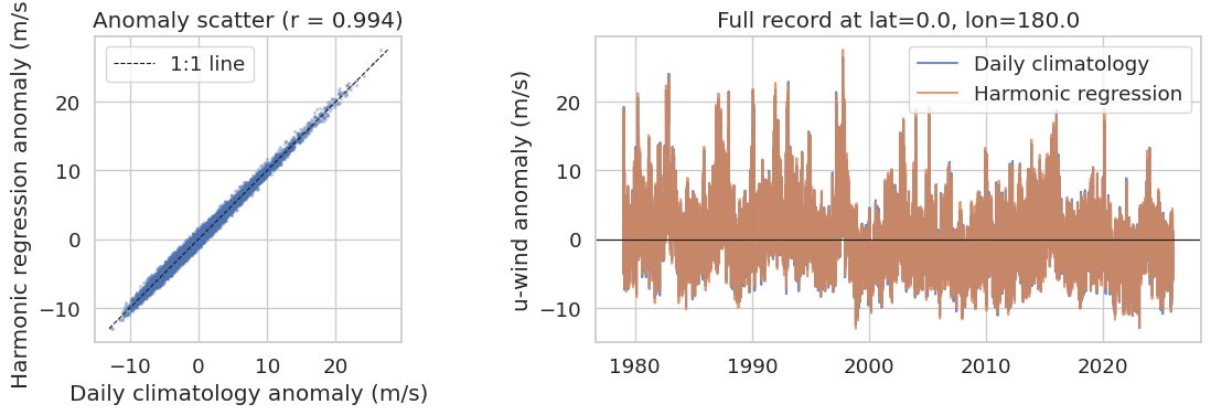
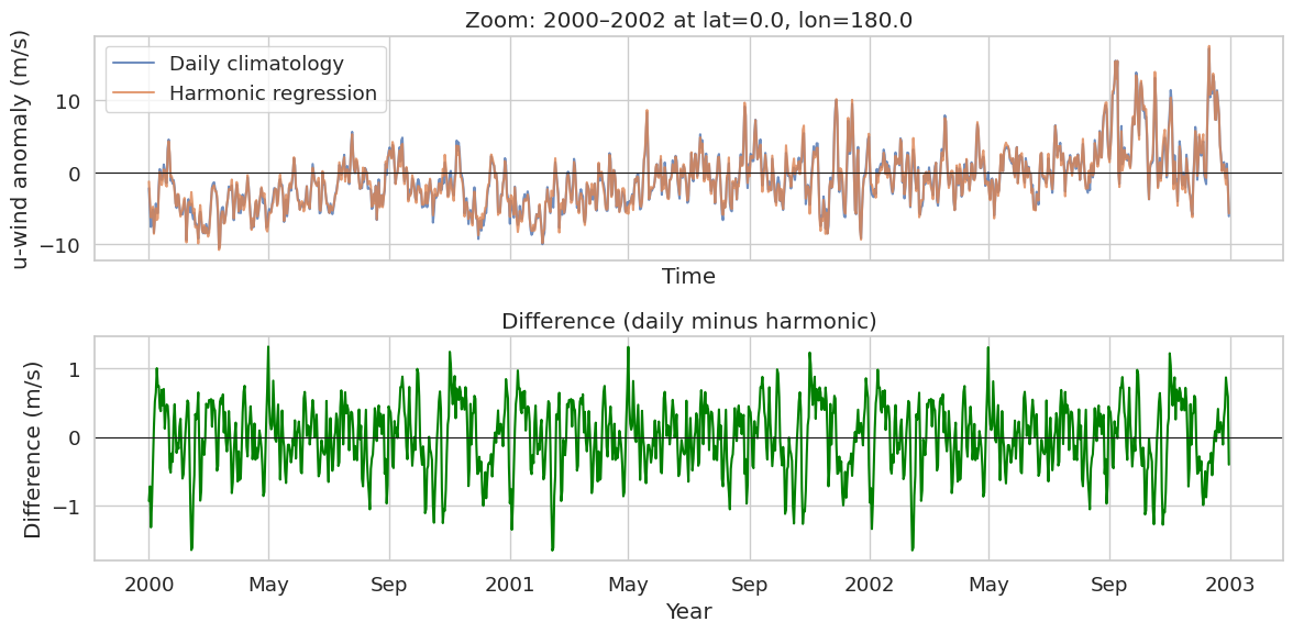
Anomalies — do the two anomaly time series track each other at a grid point and in the tropical mean?
Difference field — where and when do the methods disagree most?
Time-mean check — are anomalies near zero on average, as expected after removing the seasonal cycle?

We use the equatorial date line (0°N, 180°E) as a representative tropical grid point throughout. Lets first see how the anomalies fields look like for a particular date:

# Selecting a point on the equator
lat_select = 0.0
lon_select = 180.0
time_idx = 10

fig, axes = plt.subplots(1, 2, figsize=(14, 4),
                         subplot_kw={"projection":
                             ccrs.PlateCarree(central_longitude=180)},)
daily_anom.isel(time=time_idx).compute().plot(ax=axes[0])
axes[0].scatter(lon_select, lat_select, s=80, marker="<", color="magenta",
                transform=ccrs.PlateCarree(), label="Selected point")
axes[0].legend()
axes[0].set_title(
    f"Daily climatology anomaly\n"
    f"({pd.to_datetime(daily_anom.time[time_idx].values):%Y-%m-%d})"
)
axes[0].coastlines()
axes[0].set_aspect("auto")



harmonic_anom.isel(time=time_idx).compute().plot(ax=axes[1])

axes[1].scatter(lon_select, lat_select, s=80, marker="<", color="magenta",
                transform=ccrs.PlateCarree())
axes[1].set_title(
    f"Harmonic regression anomaly\n"
    f"({pd.to_datetime(harmonic_anom.time[time_idx].values):%Y-%m-%d})"
)
axes[1].coastlines()
axes[1].set_aspect("auto")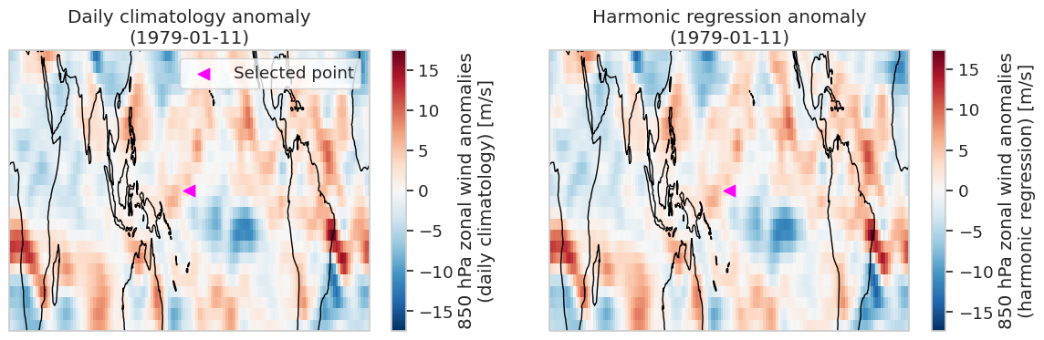

u_point = uwind_850_da.sel(
    lat=lat_select, lon=lon_select, method="nearest"
).sel(time=daily_anom.time)
daily_point = daily_anom.sel(lat=lat_select, lon=lon_select, method="nearest")
harmonic_point = harmonic_anom.sel(
    lat=lat_select, lon=lon_select, method="nearest"
)
difference_point = difference.sel(
    lat=lat_select, lon=lon_select, method="nearest"
)

# Seasonal component = original minus anomaly
seasonal_daily_pt = (u_point - daily_point).compute()
seasonal_harm_pt = (u_point - harmonic_point).compute()
doy = daily_anom.time.dt.dayofyear

fig, ax = plt.subplots(figsize=(10, 4))
seasonal_daily_pt.groupby(doy).mean().compute().plot(
    ax=ax, label="Daily climatology", alpha=0.9
)
seasonal_harm_pt.groupby(doy).mean().compute().plot(
    ax=ax, label="Harmonic regression", alpha=0.9
)
ax.set_xlabel("Day of year")
ax.set_ylabel("Seasonal $u_{850}$ (m/s)")
ax.set_title(
    f"Mean annual cycle at lat={lat_select}, lon={lon_select} "
    "(averaged over all years)"
)
ax.legend()
plt.tight_layout()
plt.show()

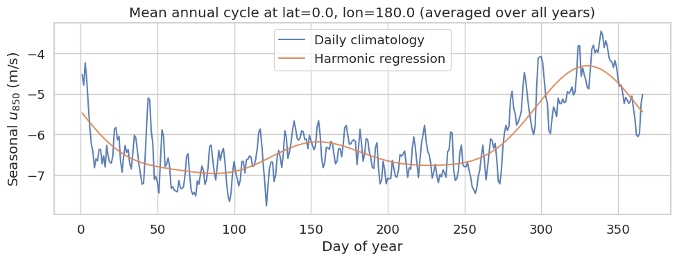
The two seasonal cycles have the same overall shape, but the daily climatology trace is jagged: each calendar day is averaged over only ~45 years, so sampling noise remains. Harmonic regression enforces a smooth annual curve and tends to sit between the day-to-day wiggles of the empirical climatology.

fig, axes = plt.subplots(1, 2, figsize=(12, 4))

x = daily_point.compute().values
y = harmonic_point.compute().values

axes[0].scatter(x, y, s=2, alpha=0.25, c="C0")
lims = [
    min(x.min(), y.min()),
    max(x.max(), y.max()),
]
axes[0].plot(lims, lims, "k--", linewidth=0.8, label="1:1 line")
point_corr = np.corrcoef(x, y)[0, 1]
axes[0].set_xlabel("Daily climatology anomaly (m/s)")
axes[0].set_ylabel("Harmonic regression anomaly (m/s)")
axes[0].set_title(f"Anomaly scatter (r = {point_corr:.3f})")
axes[0].legend()
axes[0].set_aspect("equal", adjustable="box")

axes[1].plot(daily_point.time, x, label="Daily climatology", alpha=0.8)
axes[1].plot(harmonic_point.time, y, label="Harmonic regression", alpha=0.8)
axes[1].axhline(0, color="k", linewidth=0.8)
axes[1].set_title(
    f"Full record at lat={lat_select}, lon={lon_select}"
)
axes[1].set_ylabel("u-wind anomaly (m/s)")
axes[1].legend()
plt.tight_layout()
plt.show()

fig, axes = plt.subplots(2, 1, figsize=(12, 6), sharex=True)

daily_point.sel(time=slice("2000-01-01", "2002-12-31")).plot(
    ax=axes[0], label="Daily climatology", alpha=0.8
)
harmonic_point.sel(time=slice("2000-01-01", "2002-12-31")).plot(
    ax=axes[0], label="Harmonic regression", alpha=0.8
)
axes[0].axhline(0, color="k", linewidth=0.8)
axes[0].set_title(f"Zoom: 2000–2002 at lat={lat_select}, lon={lon_select}")
axes[0].set_ylabel("u-wind anomaly (m/s)")
axes[0].legend()

difference_point.sel(time=slice("2000-01-01", "2002-12-31")).plot(ax=axes[1], color="green")
axes[1].axhline(0, color="k", linewidth=0.8)
axes[1].set_title("Difference (daily minus harmonic)")
axes[1].set_ylabel("Difference (m/s)")
axes[1].set_xlabel("Year")
plt.tight_layout()
plt.show()

fig, axes = plt.subplots(1, 2, figsize=(14, 4), subplot_kw={
                         "projection":
                             ccrs.PlateCarree(central_longitude=180)},)

daily_anom.mean("time").compute().plot(ax=axes[0], cmap="RdBu_r", add_colorbar=True)
axes[0].scatter(lon_select, lat_select, s=80, marker="<", color="magenta",
                transform=ccrs.PlateCarree(), label="Selected point")
axes[0].legend()
axes[0].set_title("Time mean: daily climatology (m/s)")
axes[0].coastlines()
axes[0].set_aspect("auto")

harmonic_anom.mean("time").compute().plot(ax=axes[1], cmap="RdBu_r", add_colorbar=True)
axes[1].scatter(lon_select, lat_select, s=80, marker="<", color="magenta",
                transform=ccrs.PlateCarree(), label="Selected point")
axes[1].set_title("Time mean: harmonic regression (m/s)")
axes[1].coastlines()
axes[1].set_aspect("auto")

plt.tight_layout()
plt.show()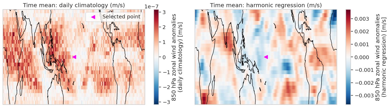

The time-mean anomaly maps should be close to zero everywhere (typically $| \bar{u}' | \ll 1$ m/s). Values near zero confirm that the seasonal cycle has been removed by both methods. Any remaining structure is much smaller than the seasonal signal itself.

Fourier analysis of monthly anomalies¶

For spectral analysis we resample to monthly means, which suppresses day-to-day noise. We remove the seasonal cycle again using monthly climatology and harmonic regression (year_period=12), then compare the FFT spectra. If either daily method left residual seasonal power, it would appear as peaks near 12, 6, 4, or 3 months; a cleaner anomaly series shows less power at those periods.

# Monthly mean zonal wind
uwind_850_monthly = (
    uwind_850_da
    .resample(time="MS")
    .mean()
    .chunk({"time": -1, "lat": 10, "lon": -1})
)

monthly_clim = uwind_850_monthly.groupby("time.month").mean("time")
monthly_clim_anom = uwind_850_monthly.groupby("time.month") - monthly_clim

# Monthly climatology and anomalies
uwind_850_clim = uwind_850_monthly.groupby("time.month").mean()
uwind_850_anom = uwind_850_monthly.groupby("time.month") - uwind_850_clim

# Time series at the selected location
uwind_850_series = uwind_850_monthly.sel(
    lat=lat_select,
    lon=lon_select,
    method="nearest",
)

monthly_harm_anom = remove_seasonal_cycle_harmonic(
    uwind_850_monthly, n_harmonics=4, year_period=12
)


monthly_clim_anom, monthly_harm_anom = dask.persist(
        monthly_clim_anom, monthly_harm_anom)

# 
monthly_clim_anom_at_point = uwind_850_anom.sel(
    lat=lat_select, lon=lon_select, method="nearest"
)
monthly_harm_anom_at_point = monthly_harm_anom.sel(
    lat=lat_select, lon=lon_select, method="nearest"
)
monthly_clim_at_point = uwind_850_series.groupby("time.month").mean("time")

fig, axes = plt.subplots(1, 2, figsize=(12, 4))
uwind_850_series.compute().plot(ax=axes[0])
axes[0].set_title(f"Monthly mean $u_{{850}}$ at lat={lat_select}, lon={lon_select}")
monthly_clim_at_point.compute().plot(ax=axes[1], marker="o")
axes[1].set_title("Monthly climatology at selected point")
axes[1].set_xticks(np.arange(1, 13))
plt.tight_layout()
plt.show()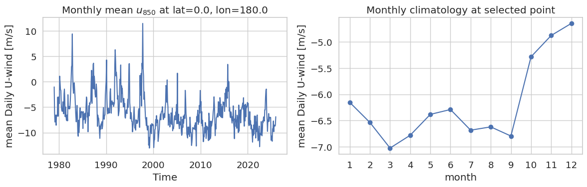

def fft_percent_variance(series, sampling_interval=1):
    """Return positive periods (months) and percent variance explained."""
    
    centered = series - np.mean(series)
    n = len(centered)
    freqs = np.fft.fftfreq(n, d=sampling_interval)
    coeffs = np.fft.fft(centered)
    power = np.abs(coeffs) ** 2
    pct = (power / np.sum(power)) * 100.0

    periods = 1 / freqs
    mask = np.isfinite(periods) & (periods > 0) & (pct > 0)
    sort_idx = np.argsort(periods[mask])
    return periods[mask][sort_idx], pct[mask][sort_idx]


def seasonal_band_power(periods, pct, ref_periods=(12, 6, 4, 3), window=0.5):
    """Sum percent variance within a window of each reference period."""
    total = 0.0
    for ref in ref_periods:
        band = (periods >= ref - window) & (periods <= ref + window)
        total += pct[band].sum()
    return total


clim_periods, clim_pct = fft_percent_variance(
    monthly_clim_anom_at_point.compute().values)
harm_periods, harm_pct = fft_percent_variance(
    monthly_harm_anom_at_point.compute().values)

clim_seasonal = seasonal_band_power(clim_periods, clim_pct)
harm_seasonal = seasonal_band_power(harm_periods, harm_pct)



print(
    f"Variance near annual harmonics (12, 6, 4, 3 mo): "
    f"monthly clim = {clim_seasonal:.2f}%, "
    f"harmonic = {harm_seasonal:.2f}%"
)

Variance near annual harmonics (12, 6, 4, 3 mo): monthly clim = 5.10%, harmonic = 5.09%

/tmp/ipykernel_4652/15789573.py:11: RuntimeWarning: divide by zero encountered in divide
  periods = 1 / freqs

fig, ax = plt.subplots(figsize=(8, 4))
ax.semilogx(clim_periods, clim_pct, label="Monthly climatology anomalies")
ax.semilogx(harm_periods, harm_pct, label="Harmonic regression anomalies",
            alpha=0.8)
reference_periods = [12, 6, 4, 3] # months
for period in reference_periods:
    ax.axvline(period, color="gray", linestyle="--", linewidth=0.8, zorder=0)
ax.set_xlabel("Period (years)")
ax.set_ylabel("Percent variance explained (%)")
ax.set_title(f"Fourier spectrum at lat={lat_select}, lon={lon_select}")
ax.legend()
ax.grid(True, which="both", alpha=0.3)

period_ticks = np.array([1/4, 1/3, 1/2, 1, 2, 3, 5, 7, 10, 15, 20])
period_ticks_months = period_ticks*12 # convert to months
period_ticks_years = [r'$\frac{1}{4}$', r'$\frac{1}{3}$', r'$\frac{1}{2}$',
                      '1', '2', '3', '5', '7', '10', '15', '20']
ax.set_xticks(period_ticks_months, period_ticks_years)

plt.tight_layout()
plt.show()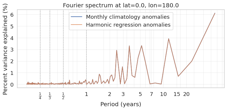

Vertical dashed lines mark the annual cycle (12 months) and its harmonics. After removing the seasonal cycle, power at those periods should be small for both methods. Remaining peaks at longer periods reflect interannual and decadal variability; the two spectra should be similar if the daily methods agreed. Lower power in the harmonic curve near 12 months often indicates a cleaner removal of the annual cycle.

Summary¶

We compared daily climatology and harmonic regression for removing the seasonal cycle from 850-hPa zonal wind.

Both methods are suitable for tropical wind analysis when the record is long. Harmonic regression is preferable when a smooth seasonal cycle is desired or the record is short. Daily climatology is simpler and needs no choice of $N$ , but its day-to-day noise propagates into the anomalies.

What’s next?¶

The next notebook, Frequency Decomposition of Zonal Wind Variability Using the Fourier Transform, extends this idea: it partitions the total variance of $u_{850}$ into annual, intraseasonal, interannual, background, and subseasonal bands and maps the spatial structure of each.

References¶

Kanamitsu, M., Ebisuzaki, W., Woollen, J., Yang, S.-K., Hnilo, J. J., Fiorino, M., & Potter, G. L. (2002). Ncep–doe amip-ii reanalysis (r-2). Bulletin of the American Meteorological Society, 83(11), 1631–1644.
Kalnay, E., Kanamitsu, M., Kistler, R., Collins, W., Deaven, D., Gandin, L., Iredell, M., Saha, S., White, G., Woollen, J., & others. (2018). The NCEP/NCAR 40-year reanalysis project. In Renewable energy (p. Vol1_146-Vol1_194). Routledge.