Spectral Preprocessing for Machine Learning: Forecasting Subseasonal Zonal Wind from OLR
Overview
Spectral preprocessing can shape what a machine-learning model learns from geophysical fields. This notebook applies a simple neural network (NN) to predict 850-hPa zonal wind near Nairobi, Kenya from outgoing longwave radiation (OLR) Lee & others, 2014 over the Indian Ocean, using a 14-day lead time.
The planned workflow is:
Load and preprocess OLR and zonal-wind fields.
Align predictors and predictand in time and inspect their power spectra.
Apply a Fourier bandpass filter to isolate intraseasonal variability.
Train and evaluate NN models on raw and bandpass-filtered OLR, with and without removing the seasonal cycle.
The goal is to compare how spectral filtering and anomaly calculation affect predictive skill, not to build a production forecast system.
Prerequisites
| Concepts | Importance | Notes |
|---|---|---|
| Fourier Power Spectrum and Spectral Filtering | Necessary | Bandpass filtering in the frequency domain |
| Remove the seasonal cycle using harmonic regression | Helpful | Harmonic anomaly approach (in progress below) |
| Removing the Seasonal Cycle: Daily Climatology vs. Harmonic Regression | Helpful | Daily-climatology anomalies used in the current workflow |
| Mapping Modes of Variability: Regressing Fields onto a Pair of Indices (MJO/RMM Example) | Helpful | OLR preprocessing context for tropical variability |
Time to learn: TBD (notebook under construction)
System requirements: TensorFlow and scikit-learn (see Imports below)
Imports
Visualization, array, and cloud I/O libraries match other application notebooks in this cookbook. TensorFlow/Keras and scikit-learn support the simple feed-forward NN and feature scaling.
import sys
# Visualization
import matplotlib.pyplot as plt
import seaborn as sns
# Data wrangling
import numpy as np
import scipy as sp
import xarray as xr
import pandas as pd
import dask
import s3fs
# Machine learning libraries
import tensorflow as tf
from tensorflow.keras.models import Sequential
from tensorflow.keras.layers import Dense, Input
from sklearn.preprocessing import StandardScaler
from sklearn.datasets import make_classification
WARNING: All log messages before absl::InitializeLog() is called are written to STDERR
I0000 00:00:1791951476.171722 4666 port.cc:153] oneDNN custom operations are on. You may see slightly different numerical results due to floating-point round-off errors from different computation orders. To turn them off, set the environment variable `TF_ENABLE_ONEDNN_OPTS=0`.
I0000 00:00:1791951476.199888 4666 cpu_feature_guard.cc:227] This TensorFlow binary is optimized to use available CPU instructions in performance-critical operations.
To enable the following instructions: AVX512F AVX512_VNNI AVX512_BF16 AVX_VNNI, in other operations, rebuild TensorFlow with the appropriate compiler flags.
Set Up
Experiment parameters define the analysis window, a chronological train/test split, the predictor–predictand lead time, and the target location near Nairobi.
ANALYSIS_PERIOD = slice('1981-01-01', '2024-12-31')
TRAINING_PERIOD = slice('1981-01-01', '2010-12-31')
TESTING_PERIOD = slice('2011-01-01', '2024-12-31')
LEAD_TIME = 14 # Lead time between predictor and predictand
NAIROBI_COORDS = {"lat": -1.2921, "lon": 36.8219}
Data Acquisition
We combine several gridded reanalysis products: OLR and zonal wind are loaded from the public Pythia Zarr stores on Jetstream2; 2-meter temperature from GDEX is planned but not yet wired in.
2-Meter Temperature (planned)
Hourly 2-meter temperature from ERA5 (GDEX Zarr) will be resampled to daily means at Nairobi. The loading cells below are commented out pending integration.
# from dask.distributed import Client, LocalCluster
# cluster = LocalCluster(
#     n_workers=5,
#     memory_limit='8GB',
# )

# client = cluster.get_client()
# client
# # Defines path of GDEX data source
# test = slice('2022-01-01', '2024-12-31')
# GDEX_URL = 'https://osdf-director.osg-htc.org/ncar/gdex/d633000/e5.oper.an.sfc.zarr/e5.oper.an.sfc.2t.zarr'
# t2m_hourly_ds = xr.open_dataset(GDEX_URL, engine='zarr')
# t2m_hourly_ds = t2m_hourly_ds.drop_vars({'quantization_info', 'utc_date'})
# t2m_hourly_ds = t2m_hourly_ds.sel(time=test)
# t2m_hourly_nairobi_ds = t2m_hourly_ds.sel(latitude=NAIROBI_COORDS['lat'], longitude=NAIROBI_COORDS['lon'], method='nearest')
# t2m_hourly_nairobi_ds# t2m_hourly_nairobi_ds.load()# # Selects prediction target near Nairobi, Kenya and resamples to daily mean
# t2m_daily_nairobi_ds = t2m_hourly_nairobi_ds.resample(time='1D').mean(dim='time')
# t2m_daily_nairobi_ds# t2m_daily_nairobi_ds.isel(time=slice(0, 365)).VAR_2T.plot(figsize=(12, 3))
# t2m_hourly_nairobi_ds.VAR_2T.plot(figsize=(12, 3))Outgoing Longwave Radiation
Daily mean OLR comes from the NCEP–NCAR Reanalysis Zarr store on the Pythia Jetstream2 bucket.
# Defines path of NCEP/NCAR Reanalysis data source
URL = 'https://js2.jetstream-cloud.org:8001/' #Locate and read a file
fs = s3fs.S3FileSystem(anon=True, client_kwargs=dict(endpoint_url=URL))
olr_noaa_store = s3fs.S3Map(
root=f'pythia/olr_noaa.zarr',
s3=fs,
check=False
)
# Open with xarray
olr_daily_ds = xr.open_zarr(olr_noaa_store)
olr_daily_ds = olr_daily_ds.rename_vars({'__xarray_dataarray_variable__': 'olr'})
olr_daily_ds.load()
olr_daily_dsInterpolation
Missing values along time are filled with linear interpolation before the fields are aligned with the wind target.
olr_daily_ds = olr_daily_ds.chunk(dict(time=-1))
olr_daily_ds = olr_daily_ds.sortby(['lat', 'lon'])
# Fill missing data with linear interpolation of neighboring values
olr_daily_ds = olr_daily_ds.interpolate_na(dim='time', method='linear', fill_value='extrapolate')
Zonal Wind
Daily 850-hPa zonal wind is read from the preprocessed NCEP–NCAR Zarr dataset used elsewhere in this cookbook.
uwind_ncep_ncar_store = s3fs.S3Map(
    root=f'pythia/uwind-ncep-ncar.zarr',
    s3=fs,
    check=False
)

# Open with xarray
uwind_daily_ds = xr.open_zarr(uwind_ncep_ncar_store)
uwind_daily_dsInterpolation
As for OLR, gaps along time are filled with linear interpolation.
uwind_daily_ds = uwind_daily_ds
uwind_daily_ds = uwind_daily_ds.chunk(dict(time=-1))
uwind_daily_ds = uwind_daily_ds.sortby(['lat', 'lon'])
# Fill missing data with linear interpolation of neighboring values
uwind_daily_ds = uwind_daily_ds.interpolate_na(dim='time', method='linear', fill_value='extrapolate')
uwind_daily_dsTarget Definition
The predictand is 850-hPa zonal wind at the grid point nearest Nairobi (NAIROBI_COORDS).
uwind_nairobi = uwind_daily_ds.sel(NAIROBI_COORDS, method='nearest').sel(level=850)Alignment
Predictor and predictand are floored to daily timestamps, OLR is shifted back by the lead time, and the two datasets are aligned on their common time index.
# Floor the time coordinates to the day
uwind_nairobi['time'] = uwind_nairobi.time.dt.floor('D')
olr_daily_ds['time'] = olr_daily_ds.time.dt.floor('D')
# Shift the OLR data by the lead time
olr_shifted = olr_daily_ds.shift(time=-LEAD_TIME).dropna(dim='time')
# Align the two datasets
uwind_aligned, olr_aligned = xr.align(uwind_nairobi, olr_shifted, join="inner")
# Load preprocessed data into memory
uwind_aligned.load()
olr_aligned.load()Spectral Analysis
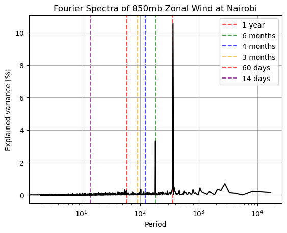
Before filtering the full OLR field, we inspect the power spectrum of the Nairobi zonal-wind time series and mark common periodicities (annual harmonics and the 14-day lead time).
def compute_power_spectrum(time_series):
    """
    Computes the normalized power spectrum (percentage of variance) of a
    time series using the Fourier transform.

    Args:
        time_series (array-like): The input time series data.

    Returns:
        tuple: (periods, percent_variance) where
            periods (np.ndarray): Array of periods corresponding to the Fourier
                frequencies.
            percent_variance (np.ndarray): Percentage of variance explained by
                each frequency component.
    """
    import numpy as np
    sampling_interval = 1
    mean_value = np.mean(time_series)
    detrended_series = time_series - mean_value

    freqs = np.fft.fftfreq(len(detrended_series), sampling_interval)
    periods = 1 / freqs

    fourier_transform = np.fft.fft(detrended_series)
    amplitude = np.abs(fourier_transform)
    power = amplitude ** 2
    normalized_power = (power / np.sum(power)) * np.var(detrended_series)
    percent_variance = (normalized_power / np.var(detrended_series)) * 100.0

    return periods, percent_variance

def plot_power_spectrum(series):
    """
    Plots the Fourier spectra of a time series.

    Args:
      serie (array-like): Input time series data.

    Returns:
      matplotlib.figure.Figure: The figure object containing the plot.
    """
    import matplotlib.pyplot as plt

    # Compute spectrum using the dedicated function
    periods, percent_variance = compute_power_spectrum(series)

    # Plot the magnitude of the FFT
    fig = plt.figure()
    ax = fig.add_subplot(111)
    ax.plot(periods, percent_variance * 2, color='k')
    ax.set_xscale('log', base=10)
    ax.set_xlabel('Period')
    ax.set_ylabel('Explained variance [%]')
    ax.set_title('Fourier Spectra')
    ax.grid(True)

    return fig, ax
# Compute and plot power spectrum of spatial mean
periods, pct_var = compute_power_spectrum(uwind_aligned.uwnd.values)
fig, ax = plot_power_spectrum(uwind_aligned.uwnd.values)
ax.set_title('Fourier Spectra of 850mb Zonal Wind at Nairobi')
# Mark harmonics of the annual cycle
harmonics = {
365.25: ('1 year', 'red'),
182.625: ('6 months', 'green'),
121.75: ('4 months', 'blue'),
91.3125: ('3 months', 'orange'),
60: ('60 days', 'red'),
14: ('14 days', 'purple')
}
for period, (label, color) in harmonics.items():
ax.axvline(period, color=color, linestyle='--',
label=label, zorder=0, alpha=0.7)
ax.legend()/tmp/ipykernel_4666/159285440.py:22: RuntimeWarning: divide by zero encountered in divide
periods = 1 / freqs
def bandpass_filter(series, low_period, high_period):
'''
Apply a bandpass filter to a time series using the Fourier transform.
Keeps frequencies corresponding to periods between low_period and high_period.
Parameters:
series (array-like): Input time series data.
low_period (float): Lower bound of the period (shorter period, higher frequency).
high_period (float): Upper bound of the period (longer period, lower frequency).
Returns:
np.ndarray: Filtered time series.
'''
import numpy as np
sampling_interval = 1
mean_value = np.mean(series)
detrended_series = series - mean_value
freqs = np.fft.fftfreq(len(detrended_series), sampling_interval)
# Handle division by zero
periods = np.where(freqs != 0, 1 / np.abs(freqs), np.inf)
# Keep frequencies with periods in [low_period, high_period]
filter_mask = (periods >= low_period) & (periods <= high_period)
fourier_coeffs = np.fft.fft(detrended_series)
fourier_coeffs[~filter_mask] = 0
filtered_series = np.fft.ifft(fourier_coeffs).real
filtered_series += mean_value
return filtered_series# Apply 1D filters to spatial mean
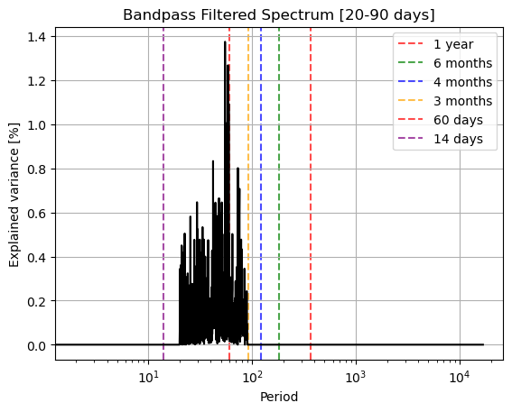
bp_low, bp_high = 20, 90
uwind_aligned_band = bandpass_filter(uwind_aligned.uwnd.values, bp_low, bp_high)
fig, ax = plot_power_spectrum(uwind_aligned_band)
# Mark harmonics of the annual cycle
harmonics = {
365.25: ('1 year', 'red'),
182.625: ('6 months', 'green'),
121.75: ('4 months', 'blue'),
91.3125: ('3 months', 'orange'),
60: ('60 days', 'red'),
14: ('14 days', 'purple')
}
for period, (label, color) in harmonics.items():
ax.axvline(period, color=color, linestyle='--',
label=label, zorder=0, alpha=0.7)
ax.legend()
ax.set_title(f'Bandpass Filtered Spectrum [{bp_low}-{bp_high} days]')/tmp/ipykernel_4666/987448014.py:21: RuntimeWarning: divide by zero encountered in divide
periods = np.where(freqs != 0, 1 / np.abs(freqs), np.inf)
/tmp/ipykernel_4666/159285440.py:22: RuntimeWarning: divide by zero encountered in divide
  periods = 1 / freqs
Filtering
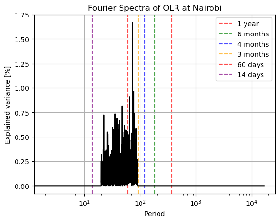
A Fourier bandpass filter (20–90 days) is applied to the gridded OLR field in parallel with Dask, isolating intraseasonal variability relevant to the MJO band Zhang, 2013.
import numpy as np
import xarray as xr

def bandpass_filter_xr(da, low_period, high_period, dim='time'):
    '''
    Apply a bandpass filter to an xarray DataArray using xr.apply_ufunc.
    Parallelized with Dask across spatial dimensions.

    Parameters:
        da (xr.DataArray): Input DataArray.
        low_period (float): Lower bound of the period.
        high_period (float): Upper bound of the period.
        dim (str): The dimension to apply the filter over.

    Returns:
        xr.DataArray: Filtered DataArray with the same dimensions.
    '''

    # FFT requires the filtering dimension to be a single continuous chunk.
    # If the data is chunked along this dimension, rechunk it to -1 (un-chunked).
    if da.chunks is not None and len(da.chunks[da.get_axis_num(dim)]) > 1:
        da = da.chunk({dim: -1})

    def _bandpass_core(array, lp, hp):
        # `apply_ufunc` moves the core dimension (dim) to the last axis (-1)
        mean_value = np.mean(array, axis=-1, keepdims=True)
        detrended = array - mean_value

        n_time = array.shape[-1]
        freqs = np.fft.fftfreq(n_time, d=1)

        # Handle division by zero
        periods = np.where(freqs != 0, 1 / np.abs(freqs), np.inf)

        # Create mask for valid frequencies
        filter_mask = (periods >= lp) & (periods <= hp)

        # Compute FFT along the last axis
        fourier_coeffs = np.fft.fft(detrended, axis=-1)

        # Apply mask (broadcasting ~filter_mask across the N-D array)
        fourier_coeffs[..., ~filter_mask] = 0

        # Compute inverse FFT and add the mean back
        filtered = np.fft.ifft(fourier_coeffs, axis=-1).real
        return filtered + mean_value

    # Apply the native numpy function across the dask array
    result = xr.apply_ufunc(
        _bandpass_core,
        da,
        kwargs={'lp': low_period, 'hp': high_period},
        input_core_dims=[[dim]],
        output_core_dims=[[dim]],
        vectorize=False,          # Set to False because our core function handles N-D arrays
        dask='parallelized',      # Use Dask to map the function over chunks in parallel
        output_dtypes=[da.dtype]
    )

    return result.transpose('time', 'lat', 'lon')

# Apply filter to OLR spatial map
filtered_olr = bandpass_filter_xr(olr_aligned['olr'],
                                  low_period=20,
                                  high_period=90)
/tmp/ipykernel_4666/1914965674.py:33: RuntimeWarning: divide by zero encountered in divide
periods = np.where(freqs != 0, 1 / np.abs(freqs), np.inf)
# Compute and plot power spectrum of spatial mean
nairobi_olr = filtered_olr.sel(NAIROBI_COORDS, method='nearest')
periods, pct_var = compute_power_spectrum(nairobi_olr.values)

fig, ax = plot_power_spectrum(nairobi_olr.values)
ax.set_title('Fourier Spectra of OLR at Nairobi')

# Mark harmonics of the annual cycle
harmonics = {
    365.25: ('1 year', 'red'),
    182.625: ('6 months', 'green'),
    121.75: ('4 months', 'blue'),
    91.3125: ('3 months', 'orange'),
    60: ('60 days', 'red'),
    14: ('14 days', 'purple')
}

for period, (label, color) in harmonics.items():
    ax.axvline(period, color=color, linestyle='--',
               label=label, zorder=0, alpha=0.7)
ax.legend()
/tmp/ipykernel_4666/159285440.py:22: RuntimeWarning: divide by zero encountered in divide
periods = 1 / freqs
Unfiltered Model
A simple feed-forward NN is trained on the full OLR field (after removing the seasonal cycle with a daily climatology computed from the training period).
Train-Test Split
Predictor and predictand are split chronologically: 1981–2010 for training and 2011–2024 for testing.
# Create the predictor (X) and target (y) variables
X = olr_aligned["olr"]
y = uwind_aligned["uwnd"]

print("Shape of predictor (X):", X.shape)
print("Shape of target (y):", y.shape)
Shape of predictor (X): (16788, 25, 144)
Shape of target (y): (16788,)
# Split data into training and testing sets defined across sequential years
X_train = X.sel(time=TRAINING_PERIOD)
y_train = y.sel(time=TRAINING_PERIOD)
X_test = X.sel(time=TESTING_PERIOD)
y_test = y.sel(time=TESTING_PERIOD)

# (OPTIONAL) Split data into training and testing sets (80% train, 20% test)
# from sklearn.model_selection import train_test_split
# X_train, X_test, y_train, y_test = train_test_split(X, y, shuffle=False, test_size=0.2, random_state=42)
Anomaly Calculation
Harmonic approach (planned)
The cells below sketch harmonic-regression anomalies following Remove the seasonal cycle using harmonic regression. This path is not yet connected to the model training cells.
# def remove_seasonal_cycle_harmonic(data, n_harmonics=4, year_period=12):
#     """
#     Remove seasonal cycle using harmonic regression.

#     Parameters
#     ----------
#     data : ndarray
#         3D array with shape (time, lat, lon). No NaN values.
#     n_harmonics : int
#         Number of harmonic pairs (sin/cos) to fit (default: 4).
#     year_period : float
#         Period of the seasonal cycle in time units (default: 12 months).

#     Returns
#     -------
#     anomalies : ndarray
#         Data with seasonal cycle removed, same shape as input.
#     """
#     n_time, n_lat, n_lon = data.shape
#     data_2d = data.reshape(n_time, -1)

#     # Build design matrix: 1 constant + n_harmonics sin/cos pairs
#     t = np.arange(n_time)
#     X = np.ones((n_time, 2 * n_harmonics + 1))
#     for i in range(1, n_harmonics + 1):
#         X[:, 2*i - 1] = np.sin(i * 2 * np.pi * t / year_period)
#         X[:, 2*i] = np.cos(i * 2 * np.pi * t / year_period)

#     # Solve via least squares and subtract seasonal component
#     coeffs = np.linalg.lstsq(X, data_2d, rcond=None)[0]
#     anomalies = data_2d - X @ coeffs

#     return anomalies.reshape(n_time, n_lat, n_lon)

# olr_anom_harmon_daily_ds = remove_seasonal_cycle_harmonic(olr_daily_ds.olr.values, n_harmonics=4, year_period=365.25)
# olr_anom_harmon_daily_ds
# def remove_seasonal_cycle_harmonic_xr(da, n_harmonics=4):
# """
# Remove seasonal cycle from a DataArray using harmonic regression.
# Parameters
# ----------
# da : xr.DataArray
# DataArray with a 'time' coordinate.
# n_harmonics : int
# Number of harmonic pairs (sin/cos) to fit (default: 4).
# Returns
# -------
# anomalies : xr.DataArray
# DataArray with seasonal cycle removed.
# """
# # Rechunk the time dimension to be a single chunk
# da = da.chunk(dict(time=-1))
# time_index = len(olr_daily_ds.time)
# year_period = 365.25 # Use days in a year for the period
# # Create the design matrix
# X = np.zeros((len(da.time), 2 * n_harmonics))
# for i in range(1, n_harmonics + 1):
# X[:, 2*i-2] = np.sin(i * 2 * np.pi * time_index / year_period)
# X[:, 2*i-1] = np.cos(i * 2 * np.pi * time_index / year_period)
# # Use apply_ufunc to apply linear regression along the time dimension
# def linear_regression(y):
# # Add an intercept
# X_with_intercept = np.c_[np.ones(X.shape[0]), X]
# # Fit the model
# coeffs, _, _, _ = np.linalg.lstsq(X_with_intercept, y, rcond=None)
# # Calculate the fit
# fit = X_with_intercept @ coeffs
# return y - fit
# anomalies = xr.apply_ufunc(
# linear_regression,
# da,
# input_core_dims=[['time']],
# output_core_dims=[['time']],
# vectorize=True,
# dask="parallelized",
# output_dtypes=[da.dtype]
# )
# anomalies['time'] = da.time
# return anomalies
# olr_anom_harmon_p_daily_da = remove_seasonal_cycle_harmonic_xr(olr_daily_ds['olr'])
# olr_anom_harmon_p_daily_da# plt.pcolormesh(olr_anom_harmon_daily_ds[0, :, :], cmap='RdBu_r', vmax=100, vmin=-100)
# plt.colorbar()# olr_anom_harmon_p_daily_da# olr_anom_harmon_p_daily_da.isel(time=0).plot(cmap='RdBu_r', vmax=100, vmin=-100)# olr_anom_daily_ds.olr.isel(time=0).plot(cmap='RdBu_r', vmax=100, vmin=-100)Standard Climatology Approach
Daily climatology is computed from the training period only and subtracted from both training and test predictors to avoid leakage.
# Calculate the daily climatology from training period
climatology = X_train.groupby('time.dayofyear').mean('time')
# Calculate the training anomalies by subtracting the training climatology
X_train = X_train.groupby('time.dayofyear') - climatology
# Calculate the testing anomalies by subtracting the training climatology
X_test = X_test.groupby('time.dayofyear') - climatology
Reshaping and Scaling
Spatial dimensions are flattened and features are standardized with StandardScaler fit on the training set.
# Convert xarray DataArrays to plain NumPy arrays and flatten spatial dimensions
# Shape goes from (time, lat, lon) to (time, lat * lon)
X_train_flat = X_train.values.reshape(X_train.shape[0], -1)
X_test_flat = X_test.values.reshape(X_test.shape[0], -1)

# Extract NumPy arrays for your targets as well
y_train_np = y_train.values
y_test_np = y_test.values

print(f"Flattened X_train shape: {X_train_flat.shape}")
print(f"Flattened y_train shape: {y_train_np.shape}")

# # 1. Clean data: Ensure absolutely no NaNs are passed to the model
# # Fill any leftover spatial NaNs in features with 0 (since they are anomalies, 0 is the mean)
# X_train_clean = np.nan_to_num(X_train_flat, nan=0.0)
# X_test_clean = np.nan_to_num(X_test_flat, nan=0.0)

# # Fill any leftover NaNs in target with the target's mean
# y_train_clean = np.nan_to_num(y_train_np, nan=np.nanmean(y_train_np))
# y_test_clean = np.nan_to_num(y_test_np, nan=np.nanmean(y_test_np))


# 2. Scale features (CRITICAL for Neural Networks)
scaler = StandardScaler()
X_train_scaled = scaler.fit_transform(X_train_flat)
X_test_scaled = scaler.transform(X_test_flat)

X_train_scaled = X_train_flat
X_test_scaled = X_test_flat
Flattened X_train shape: (10957, 3600)
Flattened y_train shape: (10957,)
Modelling
A two-hidden-layer NN (ReLU activations) is trained with mean absolute error as the loss function.
# Defines the simple ANN model architecture
model = Sequential([
    Input(shape=(X_train_scaled.shape[1],)),
    Dense(32, activation='relu'), # First hidden layer
    Dense(16, activation='relu'), # Second hidden layer
    Dense(1, activation='linear') # Linear output layer for regression
])
# Compile model with desired loss fuction and evaluation metric
model.compile(
    optimizer=tf.keras.optimizers.Adam(learning_rate=0.001),
    loss='mse',
    metrics=['mae']
)
# Show model structure and parameters
model.summary()# Fits model using training dataset
print("Starting training...")
history = model.fit(
X_train_scaled, y_train_np,
epochs=50,
batch_size=32,
validation_split=0.2,
# verbose=1
verbose=0,
)
# Evaluates trained model on testing dataset
test_loss, test_mae = model.evaluate(X_test_scaled, y_test_np, verbose=0)
print(f"Test MAE: {test_mae:.4f}")Starting training...
Test MAE: 1.4968
Analysis
Training and validation loss curves, test-set MAE, and a scatter plot of predicted versus observed zonal wind summarize model performance.
# Visualization of loss values from the training history
training_loss = history.history["loss"]
validation_loss = history.history["val_loss"]
epochs = range(1, len(training_loss) + 1)

plt.figure(figsize=(8, 5))
plt.plot(epochs, training_loss, "b-", label="Training Loss")  # Blue solid line
plt.plot(epochs, validation_loss, "r-", label="Validation Loss")  # Red solid line
plt.title("Training and Validation Loss Curves")
plt.xlabel("Epochs")
plt.ylabel("Loss")
plt.legend(loc="upper right")
plt.grid(True)
plt.show()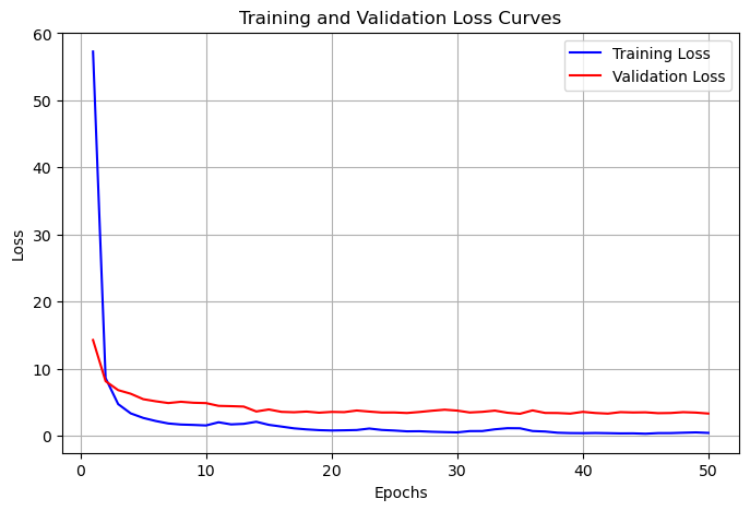
# Evaluate the model
y_pred = model.predict(X_test_scaled)
1/160 ━━━━━━━━━━━━━━━━━━━━ 3s 20ms/step140/160 ━━━━━━━━━━━━━━━━━━━━ 0s 361us/step160/160 ━━━━━━━━━━━━━━━━━━━━ 0s 503us/step
# Visualizes predicted and true values of test dataset samples
plt.figure(figsize=(6, 6))
# Scatter plot of true vs predicted values
plt.scatter(y_test, y_pred, alpha=0.5, label='Predictions')
# Generate a 1:1 line based on the data limits
# Define the slope and intercept
plt.axline((0, 0), slope=1, color='red', linestyle='--', label='1:1 Line')
# Add labels and legend
plt.xlabel('True Values (y_test_clean)')
plt.ylabel('Predictions (y_pred)')
plt.title('True vs Predicted Values')
plt.legend()
plt.grid(True, linestyle=':', alpha=0.7)
plt.show()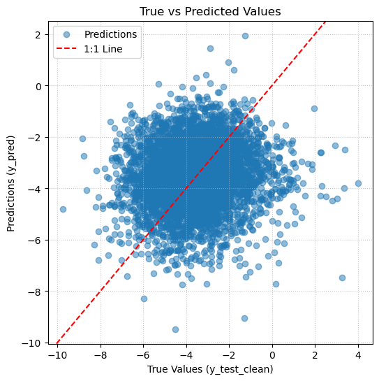
Filtered Model
The same NN architecture and preprocessing steps are repeated using bandpass-filtered OLR as the predictor, allowing a direct comparison with the unfiltered case.
Train-Test Split
Predictor and predictand are split chronologically: 1981–2010 for training and 2011–2024 for testing.
# Create the predictor (X) and target (y) variables
X = filtered_olr
y = uwind_aligned["uwnd"]

print("Shape of predictor (X):", X.shape)
print("Shape of target (y):", y.shape)
Shape of predictor (X): (16788, 25, 144)
Shape of target (y): (16788,)
# Split data into training and testing sets defined across sequential years
X_train = X.sel(time=TRAINING_PERIOD)
y_train = y.sel(time=TRAINING_PERIOD)
X_test = X.sel(time=TESTING_PERIOD)
y_test = y.sel(time=TESTING_PERIOD)

# (OPTIONAL) Split data into training and testing sets (80% train, 20% test)
# from sklearn.model_selection import train_test_split
# X_train, X_test, y_train, y_test = train_test_split(X, y, shuffle=False, test_size=0.2, random_state=42)
Standard Climatology Approach
Daily climatology is computed from the training period only and subtracted from both training and test predictors to avoid leakage.
# Calculate the daily climatology from training period
climatology = X_train.groupby('time.dayofyear').mean('time')
# Calculate the training anomalies by subtracting the training climatology
X_train = X_train.groupby('time.dayofyear') - climatology
# Calculate the testing anomalies by subtracting the training climatology
X_test = X_test.groupby('time.dayofyear') - climatology
Reshaping and Scaling
Spatial dimensions are flattened and features are standardized with StandardScaler fit on the training set.
# Convert xarray DataArrays to plain NumPy arrays and flatten spatial dimensions
# Shape goes from (time, lat, lon) to (time, lat * lon)
X_train_flat = X_train.values.reshape(X_train.shape[0], -1)
X_test_flat = X_test.values.reshape(X_test.shape[0], -1)

# Extract NumPy arrays for your targets as well
y_train_np = y_train.values
y_test_np = y_test.values

print(f"Flattened X_train shape: {X_train_flat.shape}")
print(f"Flattened y_train shape: {y_train_np.shape}")

# # 1. Clean data: Ensure absolutely no NaNs are passed to the model
# # Fill any leftover spatial NaNs in features with 0 (since they are anomalies, 0 is the mean)
# X_train_clean = np.nan_to_num(X_train_flat, nan=0.0)
# X_test_clean = np.nan_to_num(X_test_flat, nan=0.0)

# # Fill any leftover NaNs in target with the target's mean
# y_train_clean = np.nan_to_num(y_train_np, nan=np.nanmean(y_train_np))
# y_test_clean = np.nan_to_num(y_test_np, nan=np.nanmean(y_test_np))


# 2. Scale features (CRITICAL for Neural Networks)
scaler = StandardScaler()
X_train_scaled = scaler.fit_transform(X_train_flat)
X_test_scaled = scaler.transform(X_test_flat)

X_train_scaled = X_train_flat
X_test_scaled = X_test_flat
Flattened X_train shape: (10957, 3600)
Flattened y_train shape: (10957,)
Modelling
A two-hidden-layer NN (ReLU activations) is trained with mean absolute error as the loss function.
# Defines the simple NN model architecture
model = Sequential([
    Input(shape=(X_train_scaled.shape[1],)),
    Dense(32, activation='relu'), # First hidden layer
    Dense(16, activation='relu'), # Second hidden layer
    Dense(1, activation='linear') # Linear output layer for regression
])
# Compile model with desired loss fuction and evaluation metric
model.compile(
    optimizer=tf.keras.optimizers.Adam(learning_rate=0.001),
    loss='mse',
    metrics=['mae']
)
# Show model structure and parameters
model.summary()# Fits model using training dataset
print("Starting training...")
history = model.fit(
X_train_scaled, y_train_np,
epochs=50,
batch_size=32,
validation_split=0.2,
# verbose=1,
verbose=0,
)
# Evaluates trained model on testing dataset
test_loss, test_mae = model.evaluate(X_test_scaled, y_test_np, verbose=0)
print(f"Test MAE: {test_mae:.4f}")Starting training...
Test MAE: 1.4414
Analysis
Training and validation loss curves, test-set MAE, and a scatter plot of predicted versus observed zonal wind summarize model performance.
# Visualization of loss values from the training history
training_loss = history.history["loss"]
validation_loss = history.history["val_loss"]
epochs = range(1, len(training_loss) + 1)

plt.figure(figsize=(8, 5))
plt.plot(epochs, training_loss, "b-", label="Training Loss")  # Blue solid line
plt.plot(epochs, validation_loss, "r-", label="Validation Loss")  # Red solid line
plt.title("Training and Validation Loss Curves")
plt.xlabel("Epochs")
plt.ylabel("Loss")
plt.legend(loc="upper right")
plt.grid(True)
plt.show()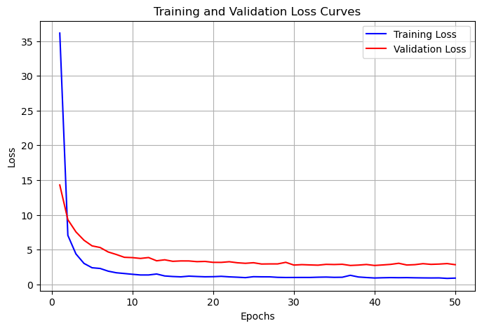
# Evaluate the model
y_pred = model.predict(X_test_scaled)
1/160 ━━━━━━━━━━━━━━━━━━━━ 2s 18ms/step160/160 ━━━━━━━━━━━━━━━━━━━━ 0s 355us/step
# Visualizes predicted and true values of test dataset samples
plt.figure(figsize=(6, 6))
# Scatter plot of true vs predicted values
plt.scatter(y_test, y_pred, alpha=0.5, label='Predictions')
plt.axline((0, 0), slope=1, color='red', linestyle='--', label='1:1 Line')
# Add labels and legend
plt.xlabel('True Values (y_test_clean)')
plt.ylabel('Predictions (y_pred)')
plt.title('True vs Predicted Values')
plt.legend()
plt.grid(True, linestyle=':', alpha=0.7)
plt.show()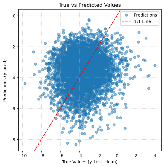
Summary
This notebook connects spectral preprocessing to a simple machine-learning forecast of local zonal wind from large-scale OLR. The full comparison between unfiltered and bandpass-filtered predictors, and between climatological and harmonic anomalies, is still being completed.
What’s next?
When this chapter is finished, readers will be able to judge whether intraseasonal filtering improves NN skill for this lead time and location.
Until then, see Mapping Modes of Variability: Regressing Fields onto a Pair of Indices (MJO/RMM Example) for a complete OLR-based diagnostic workflow.
- Lee, H.-T., & others. (2014). NOAA climate data record (CDR) of daily outgoing longwave radiation (OLR), version 1.2. (No Title).
- Zhang, C. (2013). Madden–Julian oscillation: Bridging weather and climate. Bulletin of the American Meteorological Society, 94(12), 1849–1870.