Frequency Decomposition of Zonal Wind Variability Using the Fourier Transform
Overview
Tropical low-level winds vary on a wide range of time scales, from the annual cycle driven by solar forcing, to intraseasonal fluctuations associated with the Madden–Julian Oscillation (MJO), and interannual signals linked to ENSO. A useful way to characterize a field’s variability is to partition its total variance into these time-scale bands.
In this notebook we use the Fast Fourier Transform (FFT) to decompose daily 850-hPa zonal wind () from the NCEP–NCAR Reanalysis into a set of frequency bands and map the spatial structure of each one. The workflow is:
Load daily from the public Pythia Zarr store.
Build the power spectrum at a single tropical grid point and identify the dominant peaks (annual cycle and its harmonics).
Loop over every grid point, compute the FFT, and sum the explained variance inside each band:
Annual cycle (~365 days)
Intraseasonal (20–90 days, including the MJO band)
Interannual (2–7 years, including ENSO)
Background (periods longer than 100 days)
Subseasonal (periods shorter than 80 days)
Map the explained variance (%) for each band and the total standard deviation, then interpret the resulting patterns.
The result is a set of maps showing where in the tropics each time-scale band carries most of the variability.
Prerequisites
| Concepts | Importance | Notes |
|---|---|---|
| The Discrete Fourier Transform | Necessary | Frequencies, periods, and Fourier coefficients |
| Fourier Power Spectrum and Spectral Filtering | Necessary | Power spectrum and explained variance |
| Anomaly Time Series | Helpful | Background on the same 850-hPa zonal wind dataset |
Time to learn: 20 minutes
Imports
We use xarray and s3fs to read the cloud-hosted Zarr dataset, numpy for the FFT and the band-integration math, and matplotlib/cartopy to map the variance partition.
import s3fs
import xarray as xr
import numpy as np
import matplotlib.pyplot as plt
import cartopy.crs as ccrs
import seaborn as sns

sns.set_theme(style="whitegrid", context="notebook", font_scale=1.2)
Access data
We use the same NCEP–NCAR Reanalysis Kanamitsu et al., 2002 zonal wind dataset as in Anomaly Time Series. The variable of interest is daily zonal wind, uwnd, on a global latitude–longitude grid; we will use only the lowest pressure level (level=0, 850 hPa).
URL = 'https://js2.jetstream-cloud.org:8001/' #Locate and read a file
fs = s3fs.S3FileSystem(anon=True, client_kwargs=dict(endpoint_url=URL))

uwind_ncep_ncar_store = s3fs.S3Map(
    root=f'pythia/uwind-ncep-ncar.zarr',
    s3=fs,
    check=False
)
uwind_ncep_ncar = xr.open_zarr(uwind_ncep_ncar_store)
uwind_ncep_ncarSpectral analysis
We start with a single grid point to build intuition for the FFT-based power spectrum, and then extend the same calculation to every grid point in the dataset to obtain maps of variance per frequency band.
Before carrying out the spectral analysis, let’s look at the global field on the first day of the record. The X marker indicates the eastern Indian Ocean grid point used for the single-location example below.
projPC = ccrs.PlateCarree()
fig = plt.figure(figsize=(10, 5), layout='constrained')
ax = plt.subplot(111, projection=projPC)
uwind_ncep_ncar.uwnd.isel(level=0, time=0).plot(transform=projPC, cbar_kwargs={'orientation': 'horizontal'})
ax.scatter(90, 0, marker='x', color='k', s=50, transform=projPC, zorder=3)
ax.coastlines()
ax.gridlines(draw_labels=True, alpha=0.7)
<cartopy.mpl.gridliner.Gridliner at 0x7f7dc1e255d0>/home/runner/micromamba/envs/spectral-cookbook-dev/lib/python3.11/site-packages/cartopy/io/__init__.py:263: DownloadWarning: Downloading: https://naturalearth.s3.amazonaws.com/110m_physical/ne_110m_coastline.zip
warnings.warn(f'Downloading: {url}', DownloadWarning)
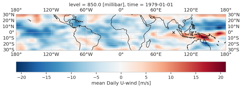
We will start by performing the FFT at a single location. We pick a grid point over the eastern Indian Ocean (0°N, 90°E), indicated by the X in the map above. This region is dominated by deep tropical convection and is a hotspot of intraseasonal variability associated with the MJO, so it is a useful place to look for energetic signals on several time scales.
uwind_ei = uwind_ncep_ncar.uwnd.isel(level=0).sel(lat=0, lon=90)
uwind_ei.plot()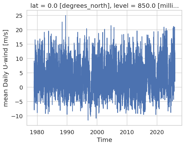
Before applying the FFT we center the series by subtracting its time mean. This removes the zero-frequency (DC) Fourier coefficient, so the spectrum describes only the variability of the time series, not its absolute level.
centered_series = uwind_ei - uwind_ei.mean(dim='time')
centered_series.plot()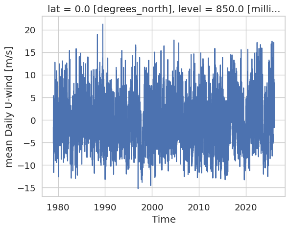
We now compute the FFT of the centered series and convert frequencies to periods with (the zero-frequency bin is set to to avoid division by zero). The power spectrum is . By Parseval’s theorem, the sum of the power equals the total variance of the series, so each bin can be expressed as the fraction of variance it explains:
sampling_interval = 1  # Assuming daily data, so 1 day between samples

freqs = np.fft.fftfreq(len(centered_series), sampling_interval)
# Handle division by zero (set zero frequency to infinity)
periods = np.where(freqs != 0, 1 / np.abs(freqs), np.inf)

# Compute Fourier coefficients and power spectrum
fourier_coeffs = np.fft.fft(centered_series)
amplitude = np.abs(fourier_coeffs)
power = (amplitude ** 2)

# Normalize power spectrum by total power and scale by series variance
normalized_power = (power/np.sum(power)) * centered_series.var().compute().values
# Total explained variance of the centered series
exp_var = (normalized_power / centered_series.var().compute().values) * 100.
/tmp/ipykernel_4458/537958354.py:5: RuntimeWarning: divide by zero encountered in divide
periods = np.where(freqs != 0, 1 / np.abs(freqs), np.inf)
plt.plot(periods,  exp_var, color='k')
plt.xscale('log')
plt.xlim(1e1, 1.5e4)
plt.ylim(1e-4, 3e0)

for period, label, color in [
    (365.25, "1 year", "C3"),
    (365.25 / 2, "6 months", "C4"),
    (365.25 / 3, "4 months", "C5"),
    (365.25 / 4, "3 months", "C6"),
]:
    plt.axvline(period, color=color, linestyle="--", alpha=0.8, label=label, zorder=1)
plt.xlabel('Days')
plt.ylabel('Explained variance [%]')
plt.title('Power spectrum of a single OLR pixel')
plt.legend()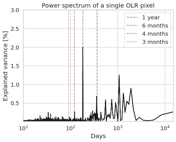
Clear spectral peaks appear at 365 days (annual cycle) and at its harmonics. Refer back to Fourier Power Spectrum and Spectral Filtering to cover this topic in depth.
We now generalize the single-point calculation to every grid point and partition the variance into a set of frequency bands. Each band is targeted at a specific kind of tropical variability:
| Band | Period range | Variability captured |
|---|---|---|
| Annual Cycle (AC) | 364–366 days | Seasonal cycle |
| Intraseasonal (IS) | 20–90 days | MJO and related convective fluctuations |
| Interannual (IA) | 2–7 years | ENSO and other low-frequency modes |
| Background (BG) | > 100 days | All low-frequency variability (includes AC and IA) |
| Subseasonal (SS) | < 80 days | All high-frequency variability (includes IS) |
For every grid point, the procedure is:
Extract the time series and center it by removing the time mean.
Compute the FFT and convert each frequency bin to its period .
Build the power spectrum and the explained-variance spectrum (% of total variance).
Apply a boolean frequency mask for each band and sum the contributions inside it.
Store both the variance (units of ) and the explained variance (%) of every band on the original spatial grid.
As a quick sanity check, we apply the annual-cycle mask to the single-point spectrum computed above. At this Indian Ocean grid point the annual band alone explains about 5.8% of the total variance:
# mask to extract different bands
ac_period = (364, 366)  # days
mask_AC = np.where((np.abs(periods) >= ac_period[0]) &
                    (periods <= ac_period[1]))

# Compute explained variances for each band
exp_var_AC = np.nansum(exp_var[mask_AC])
exp_var_ACnp.float32(0.1229185)uwind_ncep_ncar.uwnd.shape(17167, 2, 25, 144)Next, we pull the underlying NumPy array out of the xarray dataset and reshape it from (time, lat, lon) to (time, lat * lon). Collapsing the spatial dimensions into one makes it easy to iterate over grid points in a single loop.
We also allocate empty arrays — one per band — to hold the variance and the explained variance (%) at every grid point, and we set the period limits that define each band.
data_array = uwind_ncep_ncar.isel(level=0).uwnd.values

# Get the shape of the data array
dtime, dlat, dlon = data_array.shape

# Reshape data to 2D array: (time, space) for easier processing
data_reshaped = data_array.reshape(dtime, dlat * dlon)

# Variance for different frequency bands
var_AC = np.zeros(dlat * dlon) * np.nan  # Annual Cycle
var_IS = np.zeros(dlat * dlon) * np.nan  # Intra-Seasonal Cycle
var_IA = np.zeros(dlat * dlon) * np.nan  # Inter-Annual Cycle
var_BG = np.zeros(dlat * dlon) * np.nan  # Background (longer than 100 days)
var_SS = np.zeros(dlat * dlon) * np.nan  # Subseasonal (shorter than 80 days)


# Explained variance for different frequency bands
exp_var_AC = np.zeros(dlat * dlon) * np.nan  # Annual Cycle
exp_var_IS = np.zeros(dlat * dlon) * np.nan  # Intra-Seasonal
exp_var_IA = np.zeros(dlat * dlon) * np.nan  # Inter-Annual Cycle

# Background (longer than 100 days)
exp_var_BG = np.zeros(dlat * dlon) * np.nan
# Subseasonal (shorter than 80 days)
exp_var_SS = np.zeros(dlat * dlon) * np.nan

# Annual, Intra-Seasonal, Inter-annual periods in days
ac_period = (364, 366)  # days, annual cycle
is_period = (20, 90)  # days, intra-seasonal cycle
ia_period = (2*365.25, 7*365.25)  # days, inter-annual cycle

# Background and Subseasonal cutoff periods
bg_cutoff = 100  # days, background
ss_cutoff = 80  # days, subseasonal
We now loop over every grid point and repeat the single-location analysis: center the series, compute the FFT and the explained-variance spectrum, then sum the contribution of each band using the boolean masks. The results are stored in the flat (lat*lon,) arrays allocated above.
for i in range(dlat * dlon):
    # Extract time series for current gridpoint
    series = data_reshaped[:, i]

    # Define sampling interval (daily data)
    sampling_interval = 1

    # Calculate mean and center the series
    mean_value = np.mean(series)
    centered_series = series - mean_value

    # Compute FFT frequencies and convert to periods
    freqs = np.fft.fftfreq(len(centered_series), sampling_interval)
    # Handle division by zero (set zero frequency to infinity)
    periods = np.where(freqs != 0, 1 / np.abs(freqs), np.inf)

    # Compute Fourier coefficients and power spectrum
    fourier_coeffs = np.fft.fft(centered_series)
    amplitud = np.abs(fourier_coeffs)
    power = (amplitud ** 2)

    # Normalize power spectrum by total power and scale by series variance
    normalized_power = (power/np.sum(power)) * np.var(centered_series)
    # Total explained variance of the centered series
    exp_var = (normalized_power / np.var(centered_series)) * 100.

    # mask to extract different bands
    mask_AC = np.where((np.abs(periods) >= ac_period[0]) &
                       (periods <= ac_period[1]))
    mask_IS = np.where((np.abs(periods) >= is_period[0]) &
                       (periods <= is_period[1]))
    mask_IA = np.where((np.abs(periods) >= ia_period[0]) &
                       (periods <= ia_period[1]))

    mask_BG = np.where(np.abs(periods) >= bg_cutoff)
    mask_SS = np.where(np.abs(periods) <= ss_cutoff)

    # Compute variances for each band
    var_AC[i] = np.nansum(normalized_power[mask_AC])
    var_IS[i] = np.nansum(normalized_power[mask_IS])
    var_IA[i] = np.nansum(normalized_power[mask_IA])
    var_BG[i] = np.nansum(normalized_power[mask_BG])
    var_SS[i] = np.nansum(normalized_power[mask_SS])

    # Compute explained variances for each band
    exp_var_AC[i] = np.nansum(exp_var[mask_AC])
    exp_var_IS[i] = np.nansum(exp_var[mask_IS])
    exp_var_IA[i] = np.nansum(exp_var[mask_IA])
    exp_var_BG[i] = np.nansum(exp_var[mask_BG])
    exp_var_SS[i] = np.nansum(exp_var[mask_SS])
/tmp/ipykernel_4458/2317136713.py:15: RuntimeWarning: divide by zero encountered in divide
  periods = np.where(freqs != 0, 1 / np.abs(freqs), np.inf)
We reshape the flat per-grid-point arrays back to (lat, lon) so they can be plotted on a map. We also convert variances to standard deviations (the square root of the band variance), which share the same units as the original wind speeds and are easier to compare with the total standard deviation.
var_AC = var_AC.reshape(dlat, dlon)
var_IS = var_IS.reshape(dlat, dlon)
var_IA = var_IA.reshape(dlat, dlon)
var_BG = var_BG.reshape(dlat, dlon)
var_SS = var_SS.reshape(dlat, dlon)

exp_var_AC = exp_var_AC.reshape(dlat, dlon)
exp_var_IS = exp_var_IS.reshape(dlat, dlon)
exp_var_IA = exp_var_IA.reshape(dlat, dlon)
exp_var_BG = exp_var_BG.reshape(dlat, dlon)
exp_var_SS = exp_var_SS.reshape(dlat, dlon)

# Compute standard deviations
total_std = np.std(data_array, axis=0)
std_AC = np.sqrt(var_AC)
std_IS = np.sqrt(var_IS)
std_IA = np.sqrt(var_IA)
std_BG = np.sqrt(var_BG)
std_SS = np.sqrt(var_SS)Plots
With the variance partition stored on the original grid, we can now answer two complementary questions:
Where is most variable in absolute terms? — answered by the total standard deviation map.
What kind of variability dominates at each location? — answered by the explained-variance map of each band.
Total standard deviation
The map below shows the total standard deviation of daily 850-hPa zonal wind. It marks the regions where is most variable overall, without yet distinguishing between time scales. The largest values appear over the Indian Ocean and the maritime continent, consistent with the strong seasonal monsoon reversal and intense intraseasonal convective activity in that sector. Additional centers of action are found in the extratropical storm tracks of both hemispheres.
fig = plt.figure(figsize=(8, 5), layout='constrained')
ax = plt.subplot(111, projection=projPC)
plot = ax.pcolormesh(uwind_ncep_ncar.lon, uwind_ncep_ncar.lat, total_std,
                     cmap='magma',)
ax.coastlines()
ax.gridlines(draw_labels=False, alpha=0.3,)
plt.colorbar(plot, orientation='horizontal', label='Standard deviation [m/s]')
plt.title('Total Standard Deviation');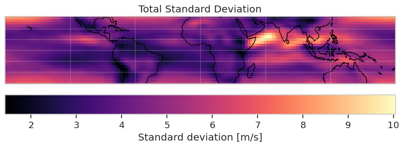
Explained variance by frequency band
The next figure shows the explained variance (%) at each grid point for the five frequency bands defined above, on a common 0–90% color scale. Bright colors indicate that the band carries most of the local variance; dark colors indicate that little of the variability lives in that band.
panels = [
    (exp_var_AC, 'Annual Cycle [364-366 days]'),
    (exp_var_IS, 'Intra-Seasonal Variability [20-90 days]'),
    (exp_var_SS, 'Subseasonal Variability [<80 days]'),
    (exp_var_BG, 'Background [>100 days]'),
    (exp_var_IA, 'Interannual Variability [2-7 years]'),
]

fig, axes = plt.subplots(
    3, 2,
    figsize=(12, 6),
    subplot_kw={'projection': projPC},
    layout='constrained',
)

for ax, (data, title) in zip(axes.flat, panels):
    plot = ax.pcolormesh(uwind_ncep_ncar.lon, uwind_ncep_ncar.lat, data,
                         cmap='viridis', vmin=0, vmax=90)
    ax.coastlines()
    ax.gridlines(draw_labels=False, alpha=0.5)
    ax.set_title(title, fontweight='bold')
    ax.set_aspect('equal')

axes.flat[-1].set_visible(False)

fig.colorbar(
    plot,
    ax=axes,
    orientation='horizontal',

    label='Explained variance (%)',
    shrink=0.6,
)
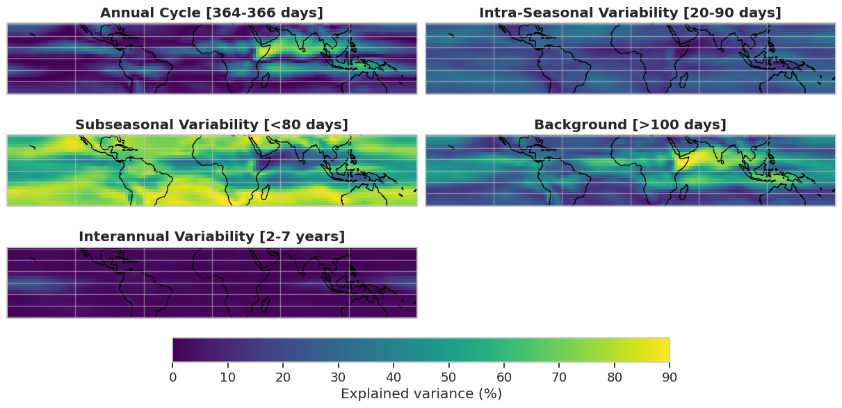
The maps highlight that different physical regimes dominate variability at different time scales:
Annual cycle (AC). The largest fraction of variance (up to ~90%) is concentrated in the monsoon belts, most notably over the Indian Ocean and the maritime continent, as well as in the African and East Asian monsoon sectors. These are the regions where the seasonal reversal of the trade winds is strongest.
Subseasonal (SS, < 80 days). Outside the monsoon belts, subseasonal variability dominates and explains a large fraction of the variance (~70% or more), particularly in the midlatitudes, where transient eddies and storm-track activity drive most of the day-to-day fluctuations.
Intraseasonal (IS, 20–90 days). A more modest contribution (~20–30%) is found within the tropical band, especially over the Indian Ocean and the western Pacific. This is the spectral fingerprint of the Madden–Julian Oscillation and related convectively coupled waves.
Interannual (IA, 2–7 years). A small but coherent contribution (a few percent) appears in the central and eastern equatorial Pacific, consistent with the imprint of ENSO on the low-level zonal flow.
Background (BG, > 100 days). This broad low-frequency envelope mirrors the AC pattern (which it contains), confirming that the annual cycle accounts for the bulk of low-frequency variability in .
Summary
In this notebook we used the Fast Fourier Transform to decompose daily NCEP–NCAR 850-hPa zonal wind into five frequency bands and mapped how each band contributes to the total variability in the tropics.
Key takeaways:
The FFT lets us go from a time series to a power spectrum; thanks to Parseval’s theorem, each frequency bin can be expressed as a fraction of the total variance.
Summing the explained variance inside a band (“integrating the spectrum”) yields the contribution of that band to the local variability, a robust way to compare time scales across regions.
For , the annual cycle dominates the monsoon belts (especially over the Indian Ocean), while the subseasonal band dominates in the midlatitudes, the intraseasonal band captures MJO activity in the tropics, and the interannual band carries an ENSO-like signal in the equatorial Pacific.
The background and subseasonal envelopes are intentionally broad and overlap with the narrower physical bands; together they confirm where low- vs. high-frequency processes account for the bulk of the variance.
What’s next?
This variance partition provides a first look at where variability occurs in frequency space. However, individual FFT frequencies can be noisy and not all peaks are statistically significant.
The next notebook, Spectral Analysis of Tropical Variability and the MJO, improves on this by using Welch’s method to smooth spectra, testing peaks against an AR(1) red-noise background, and applying a 20–90 day bandpass filter to isolate the MJO signal. It also uses lead–lag correlations and Hovmöller diagrams to examine MJO propagation and convection–circulation coupling.
A complementary approach is the EOF track (2D EOFs → 3D EOFs → Extended EOFs → Multivariate EOFs), which separates variability into spatial patterns instead of frequency bands. This method is particularly useful for identifying large-scale phenomena such as ENSO and the MJO.
- Kanamitsu, M., Ebisuzaki, W., Woollen, J., Yang, S.-K., Hnilo, J. J., Fiorino, M., & Potter, G. L. (2002). Ncep–doe amip-ii reanalysis (r-2). Bulletin of the American Meteorological Society, 83(11), 1631–1644.