Mapping Modes of Variability: Regressing Fields onto a Pair of Indices (MJO/RMM Example) - Spectral Analysis for Geophysical Data Cookbook

Overview¶

A common diagnostic in climate science is to regress a gridded field onto a pair of indices that track a particular mode of variability. The two resulting regression maps describe the spatial pattern of anomalies associated with each index; rotating between them traces the full life cycle of the mode in time and space.

In this notebook we illustrate the workflow with the Madden–Julian Oscillation (MJO): an eastward-propagating tropical disturbance characterized by large-scale anomalies in deep convection and circulation on a 20–90 day time scale Zhang, 2013.

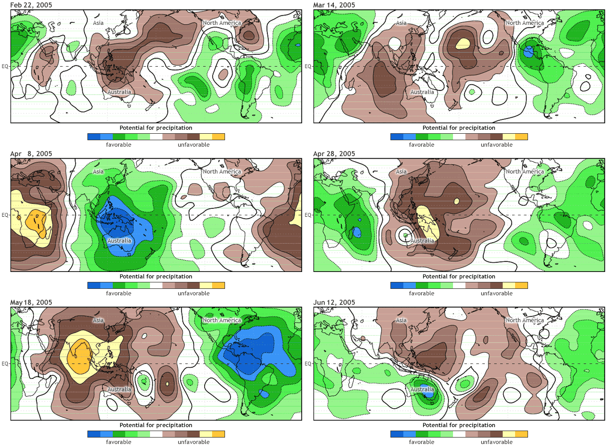
sample phase diagram — Figure 1:Example of an MJO event observed (spring 2005). Enhanced rainfall conditions (green) and suppressed rainfall conditions (brown) form a large-scale pattern that propagates eastward across the tropics. The pattern revisits a given location after approximately 45 days, illustrating the characteristic intraseasonal timescale of the MJO (Source - climate.gov).

The MJO is commonly described by the Real-time Multivariate MJO (RMM) index of Wheeler & Hendon (2004), defined as the first two principal components (RMM1 and RMM2) of equatorially averaged outgoing longwave radiation (OLR) and zonal winds at 200 and 850 hPa.

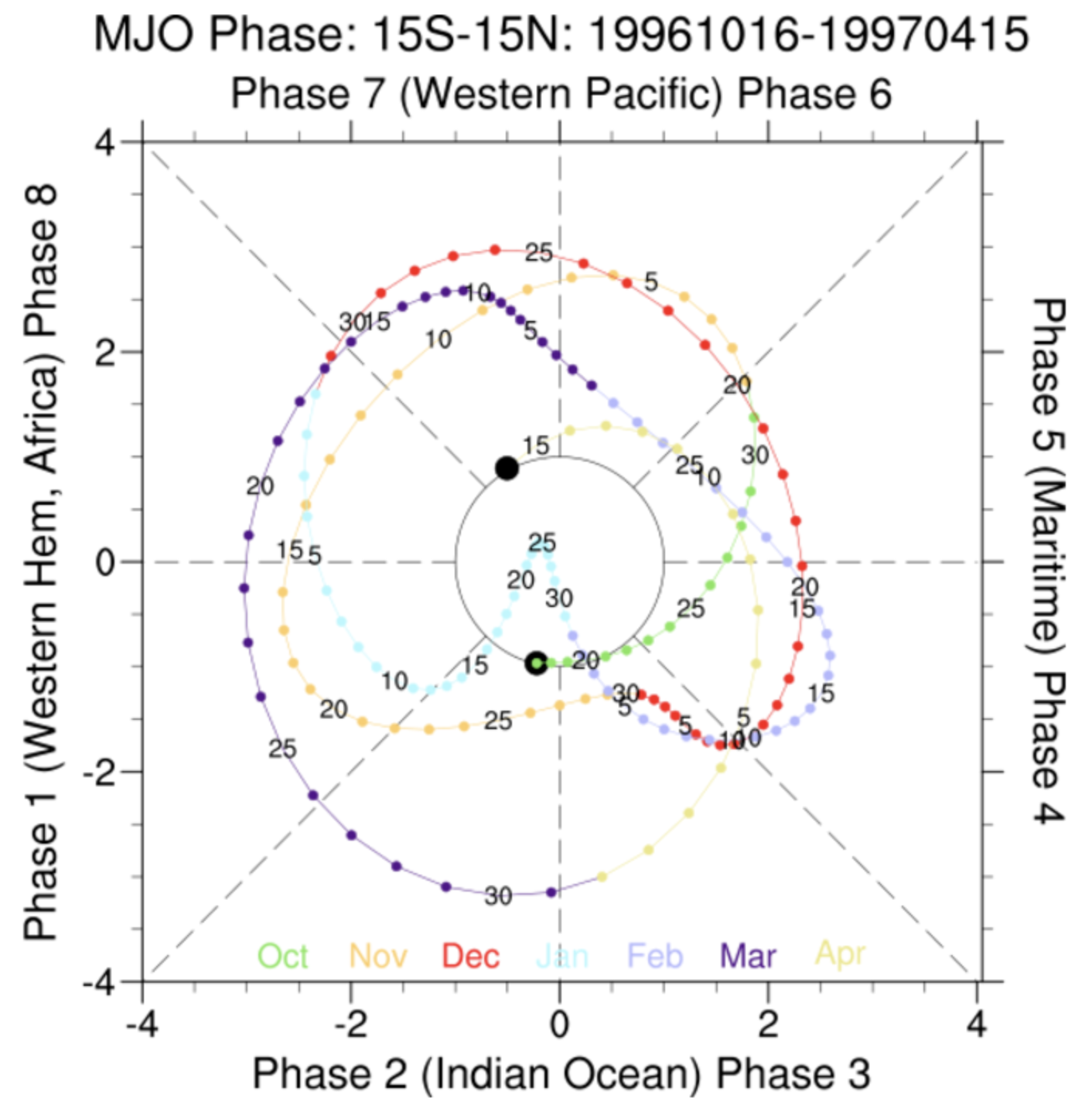
sample phase daigram — Figure 2:Example of an MJO phase daigram representing the propagation of MJO(Source-mjoclivar).

The notebook is organized as follows:

Load the observed RMM index and visualize one MJO event in RMM phase space.
Load a global OLR field and preprocess it to isolate the MJO band (fill gaps, remove the seasonal cycle, remove low-frequency variability).
Regress the preprocessed OLR onto RMM1 and RMM2 to obtain two spatial patterns.
Reconstruct the canonical MJO life cycle as linear combinations of the two regression maps.

The same recipe applies to any pair of indices and any field; only the choice of preprocessing changes.

Prerequisites¶

Concepts	Importance	Notes
Remove the seasonal cycle using harmonic regression	Necessary	Used to remove the annual cycle from OLR
3D EOFs	Helpful	Background on EOFs / principal components

Time to learn: 20 minutes

Imports¶

We use pandas to read the RMM index, xarray + s3fs to access the cloud-hosted OLR Zarr dataset, numpy for the linear algebra in the harmonic fit and the regression, and matplotlib + cartopy for visualization.

import numpy as np
import pandas as pd
import requests
from io import StringIO

import s3fs
import xarray as xr

import matplotlib.pyplot as plt
import matplotlib.dates as mdates
import cartopy.crs as ccrs
import cartopy.feature as cfeature
import seaborn as sns

sns.set_theme(style="whitegrid", context="notebook", font_scale=1.2)

Load the RMM index¶

The observed RMM index is downloaded directly from the Australian Bureau of Meteorology. Each row contains the date, RMM1, RMM2, the MJO phase (1–8), and the amplitude $\sqrt{\text{RMM1}^2 + \text{RMM2}^2}$ . If you would rather build the index from data, the Multivariate EOFs: Extracting the MJO Signal - A Simple RMM-like Index explains how to derive an equivalent RMM-like pair of PCs.

def load_rmm(url):
    """Download the Australian BOM RMM index as a DataFrame indexed by date."""
    headers = {"User-Agent": "Mozilla/5.0"}
    resp = requests.get(url, headers=headers)
    resp.raise_for_status()

    df = pd.read_csv(
        StringIO(resp.text),
        sep=r"\s+",
        header=None,
        skiprows=2,
        engine="python",
    ).iloc[:, :7]
    df.columns = ["year", "month", "day", "pc1", "pc2", "phase", "amplitude"]

    df["time"] = pd.to_datetime(df[["year", "month", "day"]])
    return df.set_index("time")[["pc1", "pc2", "phase", "amplitude"]]

url_rmm = "https://www.bom.gov.au/climate/mjo/graphics/rmm.74toRealtime.txt"
rmm = load_rmm(url_rmm)

common_start, common_end = "1990-01-01", "2024-02-24"
rmm = rmm.loc[common_start:common_end]

print(f"RMM period: {rmm.index.min().date()} to {rmm.index.max().date()}")
rmm.head()

RMM period: 1990-01-01 to 2024-02-24

Visualizing an MJO event in RMM phase space¶

A standard way to inspect the MJO is the RMM phase-space diagram: a scatter of RMM1 against RMM2, with each point representing one day. The diagram is divided into eight sectors that trace the canonical eastward progression of convection from the Indian Ocean (phases 2–3) through the Maritime Continent (phases 4–5), the western Pacific (phases 6–7), and back across the Western Hemisphere / Africa (phases 8–1). Distance from the origin is the MJO amplitude; the unit circle marks the conventional threshold for an active MJO event.

Below we focus on the DJF 2023–24 season and color the trajectory by date so the eastward propagation is visible directly.

event = rmm.loc["2023-12-01":"2024-02-24"]

fig, ax = plt.subplots(figsize=(8, 8))

ax.axhline(0, color="gray", lw=1)
ax.axvline(0, color="gray", lw=1)
ax.plot([4, -4], [4, -4], color="gray", lw=1)
ax.plot([4, -4], [-4, 4], color="gray", lw=1)
theta = np.linspace(0, 2 * np.pi, 200)
ax.plot(np.cos(theta), np.sin(theta), "k--", lw=1)

ax.plot(event["pc1"], event["pc2"], color="k", lw=1, alpha=0.5)
sc = ax.scatter(
    event["pc1"], event["pc2"],
    c=mdates.date2num(event.index),
    cmap="viridis", s=60, edgecolor="k", linewidth=0.3,
)

ax.text(0, 3.5, "W. Pacific\n(6-7)", ha="center", va="center")
ax.text(3.5, 0, "Maritime Continent\n(4-5)", ha="center", va="center", rotation="vertical")
ax.text(0, -3.5, "Indian Ocean\n(2-3)", ha="center", va="center")
ax.text(-3.5, 0, "W. Hem / Africa\n(8-1)", ha="center", va="center", rotation="vertical")

ax.set_xlim(-4, 4)
ax.set_ylim(-4, 4)
ax.set_aspect("equal")
ax.set_xlabel("RMM1")
ax.set_ylabel("RMM2")
ax.set_title("RMM phase space, DJF 2023-24")

cbar = plt.colorbar(sc, ax=ax, shrink=0.6, pad=0.08)
ticks = np.linspace(mdates.date2num(event.index[0]),
                    mdates.date2num(event.index[-1]), 5)
cbar.set_ticks(ticks)
cbar.set_ticklabels([mdates.num2date(t).strftime("%Y-%m-%d") for t in ticks])
cbar.set_label("Date")

plt.tight_layout()
plt.show()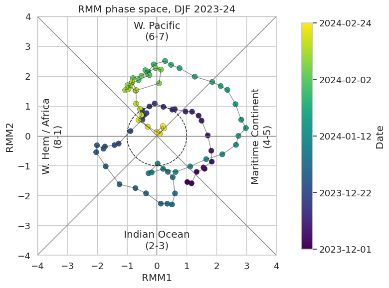

A coherent MJO event traces a counterclockwise loop through several phases while remaining outside the unit circle. The DJF 2023–24 trajectory above shows two active episodes separated by a weakening through the origin, illustrating how RMM1 and RMM2 together encode both the propagation and the strength of the MJO in just two numbers per day.

Load the OLR field¶

We use daily NOAA Outgoing Longwave Radiation (OLR) Lee & others, 2014, stored as a Zarr dataset on the Pythia Jetstream2 bucket (the same dataset used in the harmonic anomalies notebook).

URL = "https://js2.jetstream-cloud.org:8001/"
fs = s3fs.S3FileSystem(anon=True, client_kwargs=dict(endpoint_url=URL))

olr_store = s3fs.S3Map(root="pythia/olr_noaa.zarr", s3=fs, check=False)
olr_noaa = (
    xr.open_zarr(olr_store)
    .rename_vars({"__xarray_dataarray_variable__": "olr"})
    .sortby("time")
)
olr_noaa

Preprocess OLR to isolate the MJO signal¶

Before regressing onto RMM1 and RMM2, we need an OLR field that is dominated by intraseasonal (≈20–90 day) variability Zhang, 2013. Standard practice is to:

fill any missing time steps so the record is continuous,
remove the seasonal cycle, which is much larger in magnitude than the MJO,
remove low-frequency variability (e.g., ENSO-related) with a high-pass filter.

Each step is applied independently at every grid point.

Step 1: Fill missing values¶

Some days in the NOAA OLR record have no valid data anywhere on the grid. We rechunk the dataset along time and use linear interpolation to fill those gaps so the subsequent harmonic fit is well posed.

olr = (
    olr_noaa
    .chunk({"time": -1})
    .interpolate_na(dim="time", method="linear")["olr"]
)
olr

Step 2: Remove the seasonal cycle¶

The annual cycle is removed by fitting a small number of annual harmonics (sin/cos pairs) at every grid point with least squares and subtracting the fit. The full derivation is in the harmonic anomalies notebook; here we package it as a function that operates on a 3D (time, lat, lon) array.

def remove_seasonal_cycle_harmonic(data, n_harmonics=4, year_period=365.25):
    """Subtract the first ``n_harmonics`` of the annual cycle from a (time, lat, lon) array."""
    n_time, n_lat, n_lon = data.shape
    t = np.arange(n_time)

    X = np.ones((n_time, 2 * n_harmonics + 1))
    for k in range(1, n_harmonics + 1):
        X[:, 2 * k - 1] = np.sin(k * 2 * np.pi * t / year_period)
        X[:, 2 * k] = np.cos(k * 2 * np.pi * t / year_period)

    data_2d = data.reshape(n_time, -1)
    coeffs = np.linalg.lstsq(X, data_2d, rcond=None)[0]
    anomalies = data_2d - X @ coeffs
    return anomalies.reshape(n_time, n_lat, n_lon)


olr_anom = xr.DataArray(
    remove_seasonal_cycle_harmonic(olr.values, n_harmonics=4),
    coords=olr.coords,
    dims=olr.dims,
    name="olr_anom",
)

Step 3: Remove low-frequency variability¶

Even after subtracting the seasonal cycle, the anomalies still contain slow signals from ENSO and other low-frequency modes. Subtracting a 120-day centered running mean acts as a simple high-pass filter that suppresses variability with periods longer than ~120 days while preserving the 20–100 day MJO band Wheeler & Hendon, 2004.

olr_lowfreq = olr_anom.rolling(time=120, center=True).mean()
olr_mjo = olr_anom - olr_lowfreq

The plot below compares the raw OLR anomaly, the 120-day running mean, and the residual MJO-band anomaly at a Maritime Continent grid point (0°N, 120°E). The MJO-filtered series oscillates clearly on a 20–90 day time scale, with the slow drift removed.

loc = dict(lat=0.0, lon=120.0, method="nearest")

fig, axes = plt.subplots(3, 1, figsize=(10, 9), sharex=True)

olr_anom.sel(**loc).plot(ax=axes[0], color="C0")
axes[0].set_title("OLR anomaly")
axes[0].set_ylabel("OLR anomaly [W m$^{-2}$]")
axes[0].set_xlabel("")
axes[0].set_xlim(olr_anom.time[-30*365], olr_anom.time[0])

olr_lowfreq.sel(**loc).plot(ax=axes[1], color="C3", lw=2)
axes[1].set_title("120-day running mean (low-frequency)")
axes[1].set_ylabel("OLR anomaly [W m$^{-2}$]")
axes[1].set_xlabel("")
axes[1].set_xlim(olr_anom.time[-30*365], olr_anom.time[0])

olr_mjo.sel(**loc).plot(ax=axes[2], color="C2")
axes[2].set_title("MJO-band anomaly")
axes[2].set_ylabel("OLR anomaly [W m$^{-2}$]")
axes[2].set_xlim(olr_anom.time[-30*365], olr_anom.time[0])

fig.suptitle("OLR variability decomposition at 0°N, 120°E")
fig.tight_layout()
plt.show()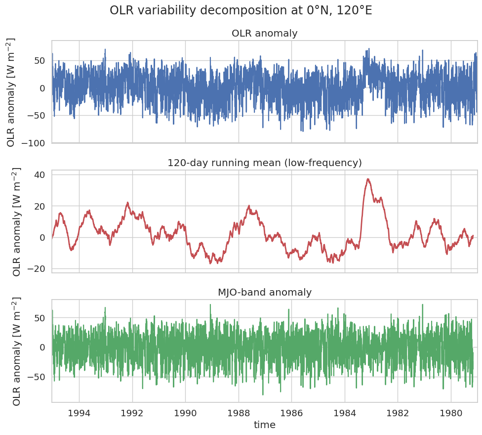

Step 4: Align the OLR field with the RMM index¶

To compute the regression, the OLR-derived time axis must match the RMM time axis exactly. We convert RMM1 and RMM2 into xarray.DataArrays, floor the OLR time stamps to daily resolution, restrict OLR to the same period, and use xr.align(..., join="inner") to keep only the common dates.

pc1 = xr.DataArray(rmm["pc1"].values, dims=["time"],
                   coords={"time": rmm.index}, name="pc1")
pc2 = xr.DataArray(rmm["pc2"].values, dims=["time"],
                   coords={"time": rmm.index}, name="pc2")

olr_mjo["time"] = olr_mjo.time.dt.floor("D")
olr_mjo = olr_mjo.sel(time=slice(common_start, common_end))

olr_mjo, pc1, pc2 = xr.align(olr_mjo, pc1, pc2, join="inner")
print(f"Aligned period: {str(olr_mjo.time.min().values)[:10]} to {str(olr_mjo.time.max().values)[:10]}")
print(f"Common samples: {olr_mjo.sizes['time']}")

Aligned period: 1990-01-01 to 2024-02-24
Common samples: 12473

Regression onto RMM1 and RMM2¶

The regression model approximates the preprocessed anomaly at every grid point as a linear combination of the two indices,

\text{OLR}'(x, y, t) \;\approx\; a(x, y)\,\text{RMM1}(t) \;+\; b(x, y)\,\text{RMM2}(t).

(1)

Because RMM1 and RMM2 are (approximately) uncorrelated and mean-zero by construction, the joint least-squares problem decouples and the two coefficients reduce to the simple univariate regression formulas

a(x, y) \;=\; \frac{\overline{\text{OLR}'(x, y, t)\,\text{RMM1}(t)}}{\overline{\text{RMM1}(t)^2}}, \qquad b(x, y) \;=\; \frac{\overline{\text{OLR}'(x, y, t)\,\text{RMM2}(t)}}{\overline{\text{RMM2}(t)^2}},

(2)

where the overlines denote time averages. Each regression map has units of OLR per unit of the corresponding index, so it can be read as the OLR anomaly that occurs (on average) when that index equals one and the other equals zero.

reg_rmm1 = (olr_mjo * pc1).mean("time") / (pc1 ** 2).mean("time")
reg_rmm2 = (olr_mjo * pc2).mean("time") / (pc2 ** 2).mean("time")

for reg in (reg_rmm1, reg_rmm2):
    reg.coords["lon"] = (((reg.lon + 180) % 360) - 180)
reg_rmm1 = reg_rmm1.sortby("lon")
reg_rmm2 = reg_rmm2.sortby("lon")

vmax = float(max(abs(reg_rmm1).max(), abs(reg_rmm2).max()))

fig, axes = plt.subplots(
    2, 1, figsize=(9, 5),
    subplot_kw={"projection": ccrs.PlateCarree()},
    constrained_layout=True, sharex=True
)
for i, (ax, data, title) in enumerate(zip(
        axes, [reg_rmm1, reg_rmm2],
        ["OLR regressed onto RMM1", "OLR regressed onto RMM2"])):
    im = data.plot(
        ax=ax, transform=ccrs.PlateCarree(),
        cmap="RdBu_r", vmin=-vmax, vmax=vmax,
        add_colorbar=False,
    )
    ax.coastlines(linewidth=0.6)
    ax.set_extent([40, 280, -30, 30], crs=ccrs.PlateCarree())
    ax.set_title(title)
    gl = ax.gridlines(alpha=0.5, draw_labels=True,)
    gl.top_labels = False
    gl.right_labels = False
    gl.bottom_labels = (i == len(axes) - 1)

cbar = fig.colorbar(im, ax=axes, orientation="horizontal",
                    shrink=0.6, extend="both")
cbar.set_label("OLR anomaly [W m$^{-2}$] per unit RMM")
plt.show()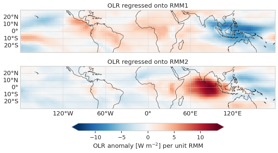

Negative values (blue) correspond to enhanced convection (more clouds, lower OLR), and positive values (red) to suppressed convection. The RMM1 map shows a dipole with enhanced convection over the Indian Ocean and suppressed convection over the western Pacific, while the RMM2 map shifts the same dipole eastward, centering the enhanced convection over the Maritime Continent and the western Pacific. Together the two maps span the equatorial belt where the MJO is active.

Reconstructing the MJO life cycle¶

A point in RMM phase space at amplitude $A$ and angle $\theta$ corresponds to $(\text{RMM1}, \text{RMM2}) = (A\cos\theta, A\sin\theta)$ . Substituting into the regression model gives the OLR anomaly expected at that point as the same linear combination of the two regression maps:

\text{OLR}'_{\theta}(x, y) \;=\; A\,\bigl[\cos\theta \cdot a(x, y) \;+\; \sin\theta \cdot b(x, y)\bigr].

(3)

Sweeping $\theta$ through evenly spaced angles reproduces the canonical MJO life cycle. Below we sample five angles that span half of phase space:

Combination	Interpretation
$-b(x, y)$	suppressed convection over the Indian Ocean
$(a - b)/\sqrt{2}$	onset of convection over the Indian Ocean
$a(x, y)$	peak convection in the Indian Ocean
$(a + b)/\sqrt{2}$	propagation toward the Maritime Continent
$b(x, y)$	mature MJO over the Maritime Continent / Western Pacific

phases = {
    r"$-\mathrm{RMM2}$": -reg_rmm2,
    r"$(\mathrm{RMM1}-\mathrm{RMM2})/\sqrt{2}$": (reg_rmm1 - reg_rmm2) / np.sqrt(2),
    r"$\mathrm{RMM1}$": reg_rmm1,
    r"$(\mathrm{RMM1}+\mathrm{RMM2})/\sqrt{2}$": (reg_rmm1 + reg_rmm2) / np.sqrt(2),
    r"$\mathrm{RMM2}$": reg_rmm2,
}

vmax = float(max(abs(p).max() for p in phases.values()))

fig, axes = plt.subplots(
    5, 1, figsize=(10, 8),
    subplot_kw={"projection": ccrs.PlateCarree()},
    constrained_layout=True,
)
for i, (ax, (title, data)) in enumerate(zip(axes, phases.items())):
    im = data.plot(
        ax=ax, transform=ccrs.PlateCarree(),
        cmap="RdBu_r", vmin=-vmax, vmax=vmax,
        add_colorbar=False,
    )
    ax.coastlines(linewidth=0.6)
    ax.add_feature(cfeature.LAND, facecolor="lightgray", alpha=0.2)
    ax.set_extent([40, 280, -30, 30], crs=ccrs.PlateCarree())
    ax.set_title(title)
    gl = ax.gridlines(alpha=0.5, draw_labels=True)
    gl.top_labels = False
    gl.right_labels = False
    gl.bottom_labels = (i == len(axes) - 1)

cbar = fig.colorbar(im, ax=axes, orientation="horizontal",
                    shrink=0.5, extend="both")
cbar.set_label("OLR anomaly [W m$^{-2}$]")
fig.suptitle("MJO life cycle from RMM regression", y=1.05)
plt.show()

/home/runner/micromamba/envs/spectral-cookbook-dev/lib/python3.11/site-packages/cartopy/io/__init__.py:242: DownloadWarning: Downloading: https://naturalearth.s3.amazonaws.com/110m_physical/ne_110m_land.zip
  warnings.warn(f'Downloading: {url}', DownloadWarning)

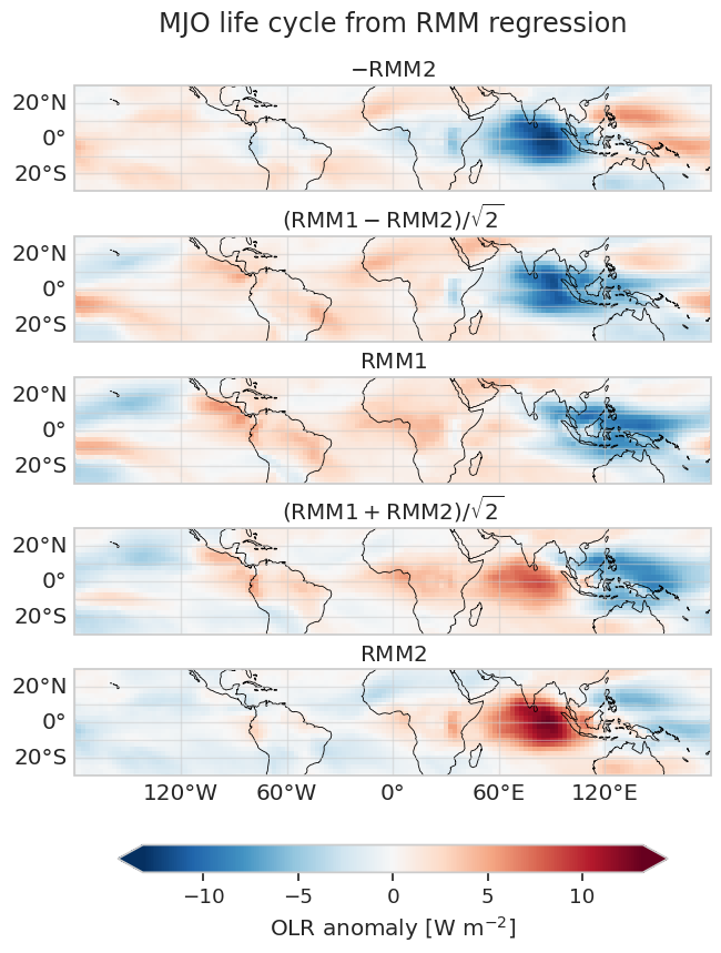
Reading the panels from top to bottom, the negative OLR anomaly (enhanced convection) shifts eastward from the Indian Ocean (RMM1) toward the Western Pacific (RMM2). This is the canonical eastward MJO propagation: a single regression onto two indices is enough to recover both basis patterns and, via simple rotations, the full eight-phase composite.

Summary¶

We regressed a preprocessed OLR field onto the two components of the RMM index to obtain a compact, physically interpretable description of the MJO. The workflow is general:

Preprocess the field to isolate the variability of interest: here, fill gaps, remove the seasonal cycle by harmonic regression, and high-pass filter with a 120-day running mean.
Align the field and the indices on a common time axis.
Regress the field onto each index using $\text{cov}(F, I)/\text{var}(I)$ at every grid point.
Reconstruct the life cycle of the mode as $\cos\theta$ / $\sin\theta$ combinations of the two regression maps.

The same recipe works for any pair of indices (e.g., ENSO-like SST PCs, annular-mode indices) and any field (precipitation, geopotential height, winds at different levels).

What’s next?¶

TBD

References¶

Zhang, C. (2013). Madden–Julian oscillation: Bridging weather and climate. Bulletin of the American Meteorological Society, 94(12), 1849–1870.
Wheeler, M. C., & Hendon, H. H. (2004). An all-season real-time multivariate MJO index: Development of an index for monitoring and prediction. Monthly Weather Review, 132(8), 1917–1932.
Lee, H.-T., & others. (2014). NOAA climate data record (CDR) of daily outgoing longwave radiation (OLR), version 1.2. (No Title).